Контур «Радоновый риск» · линия #RN4 · v9.2 · 22.07.2026

Гамма-поле короткоживущих ДПР радона в помещении: нуклид-специфичная камерная модель, Монте-Карло верификация и сверка с натурным замером

Расчёт приращения H*(10) от ²¹⁴Pb и ²¹⁴Bi на единицу ОА радона при входных величинах, восстановленных из данных эксперимента #RN3[15] (БДКГ-05), по фактической геометрии помещения. Аналитическая модель и независимый расчёт Geant4: приращение Ḣ*(10) в точке детектирования ≈ 0.59–0.64, ожидаемое показание прибора ≈ 0.75–0.76 нЗв/ч на 100 Бк/м³.

Исследование выполнено ИИ-агентами (Anthropic Claude) под руководством и контролем оператора; Монте-Карло верификация — независимым ИИ-контуром; версии статьи проходили аудит третьим ИИ-агентом. Подробности — §9 «Заявление об использовании ИИ».

Задача: связать объёмную активность ²²²Rn с приращением мощности амбиентного эквивалента дозы Ḣ*(10) гамма-излучения короткоживущих ДПР (²¹⁴Pb, ²¹⁴Bi) в точке детектирования; независимо проверить коэффициент эксперимента #RN3[15] — +1.09 нЗв/ч на 100 Бк/м³ (95 % доверительный интервал (ДИ) 1.03–1.16; собственная погрешность детектора ±20 % расширяет интервал до 0.87–1.31).

Приборы и помещение: сцинтилляционный блок детектирования БДКГ-05 (кристалл NaI(Tl) Ø40×40 мм, основная погрешность ±20 %) на стальной подставке 370×420 мм (лист 1.5 мм), центр кристалла в 1.0 м от стены, высота ~1 м; монитор радона RadonEye Plus2 на том же уровне; Г-образная комната цокольного этажа по обмерам CAD-плана (охват 5.35×9.12 м, лестничный блок 2.13×4.84 в углу, высота 2.3 м, V = 88.5 м³), бетонное перекрытие пола 30 см.

Методы: стационарная камерная модель Якоби с раздельными свободной и присоединённой фракциями и нуклид-специфичным осаждением по камерным измерениям Leonard (1994); кратность воздухообмена измерена по динамике набора радона после выключения вентиляции (0.01–0.07 ч⁻¹), скорость присоединения к аэрозолю задана по нормативному уровню запылённости (X = 25–50 ч⁻¹), коэффициент равновесия не задаётся, а вычисляется моделью (F = 0.57–0.68); перенос — прямое интегрирование ядра точечного источника по полному набору гамма-линий LNHB/DDEP (110 линий E ≥ 0.2 МэВ, ≥ 99 % гамма-энергии ДПР) с усреднением Ḣ*(10) по объёму кристалла и учётом затенения лестничным блоком; комптоновское рассеяние — модель полости с дозовым альбедо бетона по формуле Чилтона–Хаддлстона; учтены экранирование стальной столешницей и осаждение на её нижнюю плоскость. Независимая верификация — численная модель прибора и помещения в Geant4 (§5): полная геометрия блока детектирования, транспорт по тем же 110 линиям, осаждение на корпус прибора, энергетический и угловой отклик.

Вывод: вычислено приращение мощности амбиентного эквивалента дозы Ḣ*(10) на единицу ОА радона в точке детектирования; две независимые реализации согласуются: 0.59–0.64 нЗв/ч на 100 Бк/м³ (аналитическая модель) и 0.594–0.627 (Geant4). Ожидаемое показание БДКГ-05 выше этого приращения в 1.22–1.27 раза — за счёт осаждения ДПР на корпус блока детектирования (11–14 % показания) и близких осаждённых источников — и составляет 0.75–0.76 нЗв/ч на 100 Бк/м³. Измеренное в эксперименте #RN3 приращение — +1.09 нЗв/ч на 100 Бк/м³ (95 % ДИ 1.03–1.16; с инструментальной погрешностью ±20 % — суммарный интервал 0.87–1.31) — превышает вычисленное показание в 1.43–1.45 раза, а нижняя граница интервала — в 1.14–1.15 раза: расхождение выходит за пределы погрешности замера, при этом вычисление и измерение согласуются в пределах фактора 1.5 (к нижней границе интервала — в пределах 15 %). Природа расхождения рассмотрена в §6.4; инструментальный отклик его не объясняет (свёртка энергетической и угловой чувствительности по спектру ДПР — 1.004), как и неизмеренная запылённость (при коэффициенте равновесия 0.37–0.40 вычисленное показание меняется лишь на −2 %).

Ключевые слова: радон, дочерние продукты распада, ²¹⁴Pb, ²¹⁴Bi, коэффициент равновесия, осаждение аэрозолей, камерная модель Якоби, амбиентный эквивалент дозы H*(10), гамма-фон помещений, дозовое альбедо, Монте-Карло, Geant4.

1Введение

Гамма-фон, связанный с радоном, формирует не сам ²²²Rn (благородный газ, практически чистый α-излучатель на своём звене), а два звена его цепочки распада — ²¹⁴Pb (T_½ = 26.8 мин) и ²¹⁴Bi (T_½ = 19.7 мин), дающие линии от 0.24 до 2.7 МэВ. Промежуточный ²¹⁸Po (T_½ = 3.1 мин) гаммой не светит, но, осаждаясь наиболее интенсивно из всех трёх, служит основным «поставщиком» поверхностной активности гамма-эмиттеров через распад на месте.

Убыль ДПР из воздуха идёт двумя каналами с противоположным дозиметрическим следствием: вентиляция удаляет активность из помещения, тогда как осаждение сохраняет её на ограждающих поверхностях, где она продолжает излучать. Соотношение каналов задаёт коэффициент равновесия F ∈ (0, 1) и распределение дозы между воздушной и поверхностной компонентами.

Цель работы — независимая проверка коэффициента, измеренного в эксперименте #RN3: приращение мощности амбиентного эквивалента дозы +1.09 нЗв/ч на 100 Бк/м³ (95 % ДИ 1.03–1.16; сверх статистики — собственная погрешность детектора ±20 %, суммарный интервал 0.87–1.31, §6.1) при выключении вентиляции в подвале[15]. Построена расчётная модель «от первых принципов»: баланс ДПР в воздухе и на поверхностях → активности источников → перенос гамма-излучения к детектору → H*(10). Входные величины по возможности восстановлены из данных самого эксперимента: кратность воздухообмена измерена по динамике набора радона, геометрия помещения — по CAD-плану здания, геометрия стенда — по фотографии, материал подставки — по факту (сталь 1.5 мм); коэффициент равновесия при этом вычисляется моделью, а не задаётся предположением.

Проверка выполнена двумя независимыми реализациями (аналитической и Монте-Карло): аналитической моделью (камерный баланс + прямое интегрирование ядра точечного источника, §3–§4) и численным расчётом методом Монте-Карло в Geant4[19] с полной геометрией блока детектирования и помещения (§5). Второй метод дополнительно отвечает на вопросы, принципиально недоступные аналитике: вклад осаждения ДПР на корпус самого прибора и искажения его энергетического и углового отклика по спектру ДПР.

Изложение идёт от входных данных (§2) через камерную модель и перенос (§3) к результатам аналитики (§4), Монте-Карло модели прибора (§5) и сверке с натурным замером (§6).

2Исходные данные

Помещение. Г-образная комната цокольного этажа по обмерам CAD-плана здания (внутренние размеры): охватывающий прямоугольник 5.35 × 9.12 м с лестничным блоком 2.13 × 4.84 м в углу, высота 2.3 м; V = 88.5 м³, площадь пола/потолка по 38.5 м², стен — 66.6 м² (S/V = 1.62 м⁻¹). Конструктив: стена лестничного блока — кирпич 335 мм, остальные стены — бетонные блоки ФБС, все оштукатурены и оклеены флизелиновыми обоями; потолок — бетонное перекрытие; пол — паркетная доска по бетонной плите 30 см. Кирпичная стена лестничного блока (~4.7 длины свободного пробега при 0.6 МэВ) непрозрачна для гамма-излучения: часть комнаты за ней затенена и в переносе исключена.

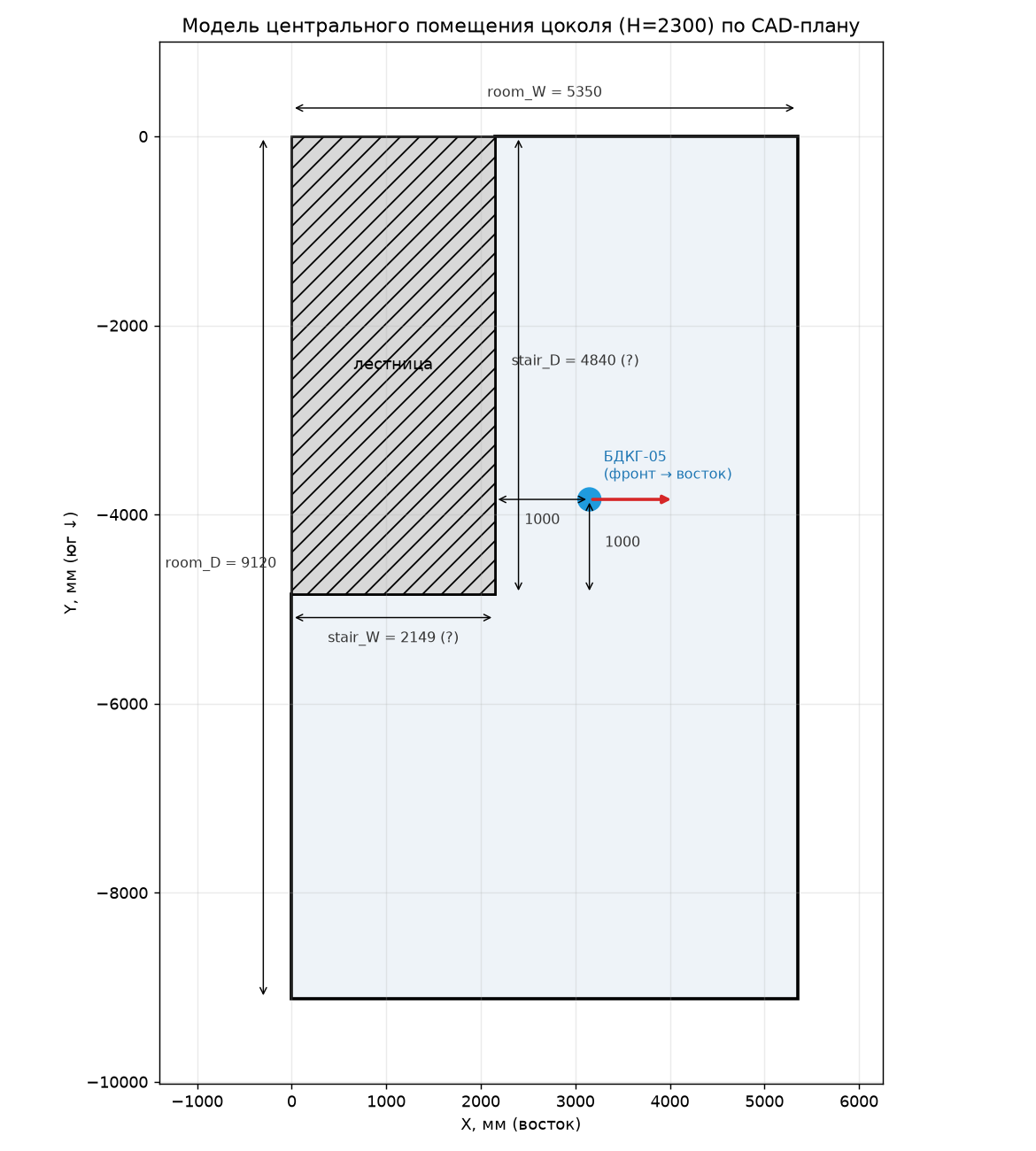
План Г-образной комнаты цоколя с позицией детектора БДКГ-05 — **Рис. 1.** План комнаты по CAD-чертежу цоколя: охват 5.35 × 9.12 м, лестничный блок (штриховка) 2.13 × 4.84 м в северо-западном углу. Детектор БДКГ-05 — в 1.0 м от стены лестничного блока и в 1.0 м от её торца, фронт на восток.

Стенд. Детектор — сцинтилляционный блок БДКГ-05 (кристалл NaI(Tl) Ø40×40 мм) на стальной подставке 370 × 420 мм (лист 1.5 мм): центр кристалла в 1.0 м от стены лестничного блока и в 1.0 м от её южного торца (Рис. 1), на высоте ≈ 1 м, ось горизонтальна (восток–запад, тыльная часть с ФЭУ обращена к стене), 3 см над столешницей. Монитор радона RadonEye Plus2 — на том же уровне.

Входные величины. Кратность воздухообмена измерена по динамике набора радона после выключения вентиляции (метод — §3.4): λ_в ≈ 0.01–0.07 ч⁻¹, в расчётах принято 0.02 ч⁻¹ — помещение в этом состоянии почти герметично. Запылённость воздуха задана по верхнему нормативному ориентиру: ПДК (предельно допустимая, а не типичная концентрация) по взвешенным частицам РМ2.5 (0.035 мг/м³ среднесуточно) для аккумуляционной моды ~0.2 мкм отвечает счётной концентрации ~5·10³–10⁴ см⁻³, то есть скорости присоединения ДПР к аэрозолю X ≈ 25–50 ч⁻¹; типичные внутренние уровни PM2.5 нередко ниже ПДК, поэтому X = 25–50 ч⁻¹ — консервативная (верхняя) оценка запылённости[2]. Скорости осаждения — прямые камерные измерения семи бытовых материалов, нормированные на стандартную комнату[4] (v_d = λ_ос·V/S, м/ч):

Таблица 1. Скорости осаждения ДПР и равновесный фактор по материалам (Leonard 1994).
Материал	`v`(²¹⁸Po)	`v`(²¹⁴Pb)	`v`(²¹⁴Bi)	F
Бетон	4.6	0.43	0.04	0.50
Дерево (лак)	5.2	0.60	0.04	0.47
Стекло	5.7	1.24	0.08	0.41
Гипсокартон	6.2	0.67	0.03	0.43
Потолочная плитка (шероховатая)	8.9	0.58	0.05	0.32
Ковёр	9.2	2.04	0.10	0.33
Штора	17.0	3.59	0.16	0.22

Привязка к геометрии: эффективной поверхностью осаждения служит поверхность контакта с воздухом, а не конструктив ограждения — потолок — бетон, стены — гипсокартон (гладкая бумажная поверхность флизелиновых обоев), пол — дерево (лак), подставка — стекло как ближайший гладкий непористый материал (для стали прямых данных нет; металл как проводник статический заряд не удерживает, электростатической составляющей осаждения нет). Для комптоновского рассеяния, напротив, обои и штукатурка радиационно прозрачны — работает субстрат (кирпич/бетон), поэтому альбедо принято бетонным. Ядерные данные: полный набор гамма-линий LNHB/DDEP[11] — 110 линий с E ≥ 0.2 МэВ и выходом ≥ 0.03 % (16 линий ²¹⁴Pb + 94 линии ²¹⁴Bi), покрывающих 99.5 % и 99.0 % гамма-энергии нуклидов (Σ E·y = 0.2217 из 0.2228 и 1.4532 из 1.4678 МэВ/распад); μ/ρ и μ_en/ρ воздуха — NIST[10]; переход керма → H*(10) — h*_K(E)[9][12].

3Методы

Расчёт разбит на три независимо контролируемых шага: баланс активностей ДПР в воздухе и на поверхностях (§3.1–§3.2), перенос излучения к точке детектирования (§3.3) и дозиметрическая свёртка; вклад каждого шага в итог линеен, контроль вычислений — §3.5.

3.1. Камерная модель ДПР

Помещение рассматривается как единая изотропно перемешанная камера (модель Якоби[1], формулировка с фракциями — Porstendörfer[2]). Стационарный баланс каждого звена цепочки:

(1)0 = λ_i·C_i−1 − (λ_i + λ_в + λ_ос,i)·C_i

Приход от распада родителя записан как λ_i·C_i−1 — с постоянной распада дочернего нуклида: C_i−1 (активность родителя) равна скорости рождения атомов дочернего, а умножение на λ_i переводит атомный баланс в баланс активностей.

Обозначения к уравнению (1). Физический смысл: приход от распада родителя = полный уход (распад + вентиляция + осаждение).
Символ	Величина	Ед.	Значение / связь
`i`	индекс звена цепочки распада	—	1 → ²¹⁸Po, 2 → ²¹⁴Pb, 3 → ²¹⁴Bi; родитель i−1 = 0 → ²²²Rn
`C`_i	объёмная активность i-го ДПР в воздухе	Бк/м³	искомая
λ_i	постоянная распада i-го нуклида	ч⁻¹	= ln2/T_½; Po 13.42, Pb 1.552, Bi 2.111
λ_в	кратность воздухообмена	ч⁻¹	измерена: 0.01–0.07; принято 0.02 (§3.4)
λ_ос,i	эффективная скорость осаждения i-го нуклида	ч⁻¹	= Σ_s v_d,i,s·A_s/V (Табл. 1)

Основная модель — полная, с раздельными свободной и присоединённой фракциями каждого ДПР: присоединение к аэрозолю со скоростью X, отрыв ²¹⁴Pb при α-распаде присоединённого ²¹⁸Po (p = 0.83[7]), нуклид- и материал-специфичное осаждение свободной фракции (Табл. 1), диффузионное осаждение присоединённой (0.1 м/ч[2]) и вертикальный член гравитационного оседания аэрозоля ±v_s (v_s = 0.012 м/ч для AMD ≈ 200 нм; пол/подставка +, потолок −). Коэффициент равновесия при этом не задаётся заранее, а вычисляется самой моделью:

(2)F = 0.105·f₁ + 0.515·f₂ + 0.380·f₃, f_i = C_i/C₀

где f_i — доля активности i-го ДПР (сумма фракций) относительно ОА радона C₀; 0.105, 0.515, 0.380 — весовые множители ЭРОА, доли потенциальной альфа-энергии на ²¹⁸Po, ²¹⁴Pb, ²¹⁴Bi (UNSCEAR 2000 Annex B, p. 103, § 122[8]).

Для граничных сценариев (ограничивающих оценку снизу) используется одногрупповое приближение (единая эффективная λ_ос,i на нуклид, без разделения фракций): F фиксируется (0.3 или 0.4), а λ_в восстанавливается обратной задачей из (2). Расхождение одногруппового приближения с полной моделью — единицы процентов (§4.4).

3.2. Поверхностная активность

Активность каждого звена на поверхности следует из стационарного баланса «осаждение из воздуха + внутриповерхностное подрастание от родителя = распад». Ключевой механизм — распад осаждённого ²¹⁸Po непосредственно на поверхности; часть новорождённого ²¹⁴Pb выбивается отдачей при α-распаде обратно в воздух (фактор отскока R[4]):

(3)A_Po = v_PoC_Po/λ_Po; A_Pb = v_PbC_Pb/λ_Pb + (1−R)·A_Po; A_Bi = v_BiC_Bi/λ_Bi + A_Pb

Вывод. В установившемся режиме приход атомов на поверхность равен их убыли: λ_доч·N_доч = v_d·n_возд + (1−R)·λ_род·N_род, где n_возд = C/λ_доч — атомная концентрация в воздухе, а λ_род·N_род = A_род (каждый распад родителя рождает один атом дочернего). Левая часть — это и есть A_доч, откуда (3). Контроль: при R = 0 и v_Pb = v_Bi = 0 формула обязана давать секулярное равновесие A_Po = A_Pb = A_Bi — тест встроен в расчётный скрипт (PASS). В полной модели приток на поверхность складывается из обеих фракций.

где A_i — поверхностные активности, Бк/м²; v_i — скорости осаждения на данную поверхность, м/ч (Табл. 1); C_i — объёмные активности в воздухе, Бк/м³; R — фактор отскока (доля ²¹⁴Pb, выбиваемая обратно в воздух при α-распаде осевшего ²¹⁸Po). Принято R = 0.5 — расчётная колонка Таблицы 1 источника[4] (теоретический максимум для плоскости); измеренные значения для материалов помещения — 0.29–0.36, бетон не измерялся (экстраполяция ~0.30). Существенно, что v_d(²¹⁴Pb) Таблицы 1 вычислены авторами в предположении R = 0.5, поэтому варьировать R можно только согласованной парой (R, v_d(Pb|R)): v_Pb(R) = v_Pb(0.5) − (0.5−R)·(v_Po/λ_Po)·(λ_Pb + v_Pb(0.5)/0.6818); контрольная точка — бетон: R = 0.3 → v_d(Pb) = 0.28 м/ч. Эффекты подрастания и прямого осаждения при этом противонаправлены и почти полностью компенсируются: итог по всему диапазону R = 0.29–0.55 меняется лишь на ±0.5 % (§4.4).

Осаждение по Якоби ≠ гравитационное оседание. «Осаждение» (λ_ос) — поток ДПР к поверхностям через приповерхностный пограничный слой, движимый диффузией (броуновской + турбулентной), а не тяжестью; оно изотропно и управляется быстрой свободной фракцией (~1 нм, v_d ≈ 5–20 м/ч). Транспорт через объём обеспечивает конвекция (5–20 см/с, оборот комнаты за десятки секунд), лимитирует последний миллиметровый погранслой: δ = D/v_d ≈ 4 мм; чистая молекулярная диффузия перенесла бы атом лишь на √(6Dτ) ≈ 9 см за время жизни. Гравитационное оседание — отдельный вертикальный механизм (v_s ≈ 0.01 м/ч, только присоединённая фракция, только горизонтали) и в итоге пренебрежимо (< 0.5 %); реальную ориентационную асимметрию задаёт естественная конвекция — вертикальные стены осаждают в ≈ 1.8 раза сильнее горизонталей[5].

3.3. Перенос и дозиметрия

Флюенс в точке детектирования — прямое интегрирование ядра точечного изотропного источника с экспоненциальным ослаблением в воздухе[13], раздельно по трём источникам (объём воздуха, грани помещения, подставка), каждый со своей активностью:

(4)G_об(E) = ∫_V e^−μr/(4πr²) dV, G_пов(E) = ∫_S e^−μr/(4πr²) dA

(5)ΔḢ*(10) = Σ_нукл Σ_линий A·y·G(E)·E·(μ_en/ρ)(E)·h*_K(E)

где G(E) — геометрические факторы объёмного (м) и поверхностного (безразмерный) источников; μ(E) — линейный коэффициент ослабления воздуха, м⁻¹; r — расстояние от элемента источника до точки расчёта; A — объёмная (Бк/м³) или поверхностная (Бк/м²) активность; y — выход линии, фотон/распад[11]; (μ_en/ρ) — массовый коэффициент поглощения энергии воздуха, м²/кг[10]; h*_K(E) — переход воздушная керма → H*(10), Зв/Гр[9][12]. Размерные множители опущены.

Модель источников. (1) Объёмный — активности ²¹⁴Pb/²¹⁴Bi равномерно по всему объёму Г-комнаты, детектор внутри. (2) Поверхностные — пол, потолок и шесть участков стен (Рис. 1), каждый со своей активностью по (3) (материал и ориентация различаются), вклады группируются «потолок / пол / стены». (3) Локальный — столешница 370×420 мм с активностью верхней плоскости; источник в сантиметрах от кристалла.

Численное интегрирование. Объём — сетка 5 см послойно; сингулярность ядра при r → 0 снимается аналитически: окрестность радиусом 15 см вокруг детектора интегрируется как равномерный шар, (1 − e^−μR)/μ. Грани — сетка 5 см (минимальное r = 1.00 м — до стены лестничного блока, сингулярности нет; осевшая активность — изотропный излучатель на единицу площади, косинусные множители не вводятся). Затенение: элементы объёма и граней без прямой видимости от детектора (за кирпичной стеной лестничного блока) исключаются; торец блока обращён от детектора и вклада не даёт. Фактор G отдельных граней при 0.609 МэВ: пол 0.519, потолок 0.418, стены суммарно 0.547, из них стена лестничного блока (1.0 м от детектора) 0.299 — 55 % вклада стен, восточная стена 0.169 — 31 %; в пределе бесконечной плоскости зависимость от расстояния лишь логарифмическая, (S_A/2)·E₁(μd), отсюда слабая чувствительность итога к точному зазору детектор–стена. Подставка — сетка 5 мм, Ḣ*(10) усредняется по объёму кристалла (сетка 4 мм, ~800 точек внутри цилиндра): в ближней зоне точечное приближение даёт заметную ошибку.

Комптоновское рассеяние — модель полости. Воздух слабо ослабляет излучение (длина свободного пробега ~80 м); непоглощённый фотон попадает на ограждение, доля a_D отражается и вновь облучает комнату; сумма переотражений даёт фактор полости B(E) = 1/(1 − a_D(E)), которым умножается доза каждой линии. Интегральное дозовое альбедо бетона a_D(E) выведено из первоисточника: формула Чилтона–Хаддлстона[16] с параметрами C, C′ МК-подгонки для толстой бетонной плиты (Табл. I[18]; обзор[17]) численно проинтегрирована по полусфере отражения, отдельно для нормального падения (нижняя оценка) и изотропного облучения стен (центральная); контроль: a_D(0.662 МэВ, 0°) = 0.063 при литературных 0.06–0.08. Поправка составляет +6 % (нормальное) … +10 % (изотропное). Ограничения подхода: рассеянная добавка позиционно-независима (позиция детектора учтена только в прямой компоненте), сумма переотражений — эвристика интегрирующей сферы; более полный учёт возможен методом Монте-Карло (как в[3]).

Стальная столешница (1.5 мм). Сквозь столешницу к кристаллу проходит 43 % направлений — 35 % воздушного геометрического фактора и весь вклад пола; лист стали ослабляет этот нижний поток на −0.020 нЗв/ч на 100 Бк/м³ (расчёт по всем 110 линиям с наклонными толщинами, NIST-данные железа). Одновременно нижняя плоскость столешницы — поверхность осаждения в ~4.5 см от кристалла, светящая сквозь ту же сталь: +0.035…+0.045 нЗв/ч на 100 Бк/м³ (активность нижней плоскости принята как у потолка — такой же обращённой вниз поверхности). Нетто-поправка +0.013…+0.028 нЗв/ч на 100 Бк/м³ входит в базовую оценку.

3.4. Измерение кратности воздухообмена

Кривая набора радона в эксперименте #RN3[15] позволяет определить λ_в. Баланс радона в перемешанном воздухе комнаты — приход от постоянного источника S (поступление грунтового газа) за вычетом убыли по двум каналам, вентиляции и собственного распада:

dC/dt = S − (λ_в + λ_Rn)·C(6)

При постоянном S концентрация выходит на баланс по экспоненте:

C(t) = C_∞ + (C₀ − C_∞)·e^{−k t}, k = λ_в + λ_Rn, C_∞ = S/(λ_в + λ_Rn)(7)

Постоянная распада радона известна точно (λ_Rn = ln2/T_½ = 0.00755 ч⁻¹), поэтому измеренная «скорость закругления» k напрямую даёт вентиляцию: λ_в = k − λ_Rn. Подгонка трёхпараметрическая: при каждом пробном k — линейный МНК по базису {1, e^{−k t}} (даёт C_∞ и C₀), выбирается k с наименьшей невязкой; 95 % интервал — по профилю невязки.

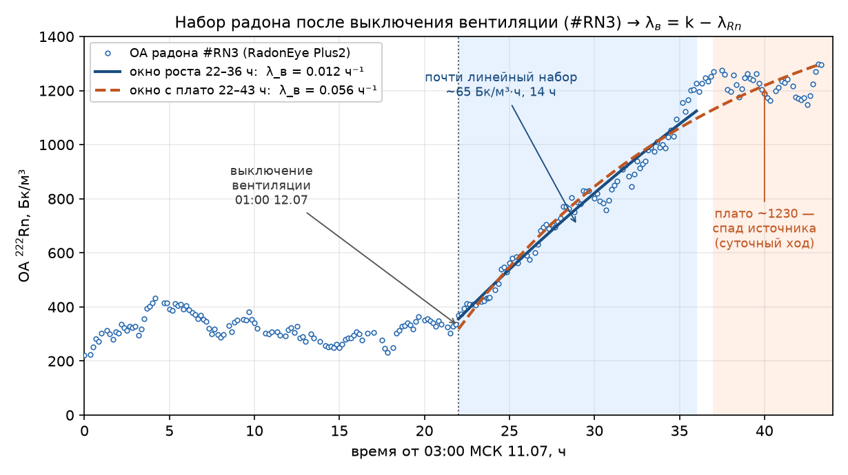
Кривая набора радона #RN3 после выключения вентиляции с двумя подгонками — **Рис. 2.** Набор ²²²Rn после выключения вентиляции (RadonEye Plus2, #RN3). До эксперимента (0–20 ч) виден суточный ход источника при работающей вентиляции. С 01:00 12.07 (x = 22 ч) — почти линейный набор ~65 Бк/м³·ч в течение 14 ч без выполаживания. Резкое плато ~1230 Бк/м³ с 16:00 — суточный спад поступления грунтового газа, а не вентиляционный баланс. Линии — подгонка ур. (7) в двух окнах.

Почти линейный рост в течение 14 часов без выполаживания — признак почти герметичного помещения: постоянная времени τ = 1/k велика по сравнению с окном наблюдения, и видна лишь ранняя, слабо изогнутая часть экспоненты. Результат подгонки зависит от того, включать ли плато:

Подгонка кривой набора в двух окнах (λ_Rn = 0.00755 ч⁻¹).
Окно подгонки	Точек	k, ч⁻¹	C_∞, Бк/м³	λ_в = k − λ_Rn, ч⁻¹
Чистый рост (22–36 ч)	79	0.020	3504 (нефизично)	0.012 [0.012–0.021]
С плато (22–43 ч)	118	0.064	1638	0.056 [0.043–0.070]

В окне чистого роста кривая почти прямая, асимптота не определяется — экстраполяция даёт нефизично высокое C_∞ ≈ 3500 Бк/м³; окно надёжно говорит лишь, что λ_в мал (≲ 0.02 ч⁻¹). В окне с плато формальная подгонка объясняет выполаживание вентиляционным балансом и поднимает λ_в до 0.056, но плато наступает резко (за ~1 ч) и точно в суточный максимум — это спад источника, а не гладкое экспоненциальное насыщение (тот же суточный ход виден и до эксперимента), поэтому 0.056 — верхняя граница. Итоговая оценка λ_в ≈ 0.01–0.07 ч⁻¹, физически — почти герметичное помещение (λ_в ≲ 0.05); лаг RadonEye ~30 мин на фоне 14-часового набора пренебрежим. В расчётах принято λ_в = 0.02 ч⁻¹; чувствительность итога к диапазону 0.01–0.05 — +0.8…−2.3 % (§4.4), поскольку при столь слабом воздухообмене баланс ДПР задаётся осаждением, а не вентиляцией. Отсюда следует, что объяснить наблюдаемое неравновесие одной вентиляцией, без осаждения, не удаётся: потребовалась бы λ_в ≈ 1.4–2.6 ч⁻¹ (§6.3).

3.5. Контроль вычислений

В расчётный скрипт встроены обязательные проверки: тест секулярного равновесия для (3) (при R = 0 и нулевом прямом осаждении A_Po = A_Pb = A_Bi; при провале — аварийный останов), контроль невязки |F − F_цель| после бисекции в решателях. Воздушная компонента дополнительно верифицирована независимой угловой квадратурой (1.28·10⁶ лучей, радиальный интеграл аналитический — сингулярности нет в принципе): совпадение с сеточным методом +0.4 %. Сходимость сеток: измельчение вдвое меняет фактор граней в 5-м знаке, подставки — на 0.04 %. Линейность дозы по ОА радона точна алгебраически и подтверждена экспериментально (v_d не зависит от ОА[6]).

4Результаты

4.1. Коэффициент равновесия, вычисленный моделью

При измеренной вентиляции коэффициент равновесия определяется запылённостью — скоростью присоединения ДПР к аэрозолю X (§3.1):

Таблица 2. Коэффициент равновесия и свободная доля ²¹⁸Po как функции запылённости (λ_в = 0.02 ч⁻¹).
X (присоединение к аэрозолю), ч⁻¹	Уровень запылённости	F (вычислен)	Свободная доля ²¹⁸Po
5	очень чистый воздух	0.30	0.73
10	чистый воздух	0.41	0.58
25	≈ ПДК РМ2.5	0.57	0.35
50	типичное жильё	0.68	0.21
100	запылённое	0.76	0.12

Базовый диапазон X = 25–50 даёт F = 0.57–0.68 (ЭРОА 57–68 Бк/м³ на 100 Бк/м³ ОА). Запылённость в помещении не измерялась, поэтому F здесь — расчётная величина при нормативном аэрозоле. Прямые измерения коэффициента равновесия в помещениях с отключённой вентиляцией дают F = 0.35–0.45[21]; в рамках модели при измеренной λ_в = 0.02 ч⁻¹ такие значения отвечают чистому воздуху (X ≈ 8–10 ч⁻¹) и рассмотрены как отдельный сценарий (§4.3, §4.4). Достичь F ≤ 0.45 вентиляцией при нормативном аэрозоле нельзя — потребовалась бы λ_в ≈ 0.7–1 ч⁻¹, исключённая измеренной динамикой набора (§3.4).

4.2. Активности в воздухе и на поверхностях

Таблица 3. Объёмная активность ДПР в воздухе (Бк/м³ на 100 Бк/м³ Rn; сумма свободной и присоединённой фракций). X — скорость присоединения ДПР к аэрозолю, ч⁻¹ (§3.1): 25 — норматив запылённости, 50 — типичное жильё.
Нуклид	X = 25	X = 50
²¹⁸Po	80.4	86.7
²¹⁴Pb	56.2	67.9
²¹⁴Bi	51.0	62.3

Таблица 4. Поверхностная активность ²¹⁴Pb / ²¹⁴Bi (Бк/м² на 100 Бк/м³ Rn). X — скорость присоединения к аэрозолю, ч⁻¹ (§3.1).
Поверхность	X = 25		X = 50
Поверхность	²¹⁴Pb	²¹⁴Bi	²¹⁴Pb	²¹⁴Bi
Потолок (бетон)	19.2	21.7	14.1	16.9
Стены (обои)	25.5	28.4	18.4	21.5
Пол (паркет)	22.2	25.4	16.6	20.1
Подставка (сталь)	23.1	26.3	17.1	20.6

Рост запылённости перераспределяет активность с поверхностей в воздух: аэрозоль перехватывает ²¹⁸Po до осаждения (свободная доля 0.35 → 0.21), поверхностное подрастание гаснет, воздушные ²¹⁴Pb/²¹⁴Bi растут. В точке измерения эти сдвиги почти компенсируются в дозе (§4.4).

4.3. Мощность дозы

Таблица 5. Приращение ΔḢ*(10) по компонентам и базовая оценка (нЗв/ч на 100 Бк/м³ Rn). X — скорость присоединения к аэрозолю, ч⁻¹ (§3.1).
Компонента	X = 25	X = 50
Воздух комнаты	0.332	0.405
Потолок (бетон)	0.027	0.021
Стены (обои)	0.047	0.035
Пол (паркет)	0.040	0.031
Подставка (сталь, верх)	0.081	0.063
Прямые фотоны, итого	0.527	0.555
+ комптон (изотропное альбедо)	0.579	0.610
+ столешница (экран −0.020; нижняя плоскость +0.035…+0.045)	+0.015…+0.025	+0.015…+0.025
Базовая оценка приращения Ḣ*(10)	0.59–0.60	0.63–0.64

Базовая оценка приращения Ḣ*(10): 0.59–0.64 нЗв/ч на 100 Бк/м³, центральное значение ≈ 0.61. При высоком равновесии доминирует воздушная компонента (63–73 % прямых фотонов); подставка — крупнейший единичный поверхностный источник (большой телесный угол вплотную к кристаллу). Это оценка приращения Ḣ*(10) — без инструментальных эффектов самого прибора (осаждение на корпус, §5); альбедо-модель полости даёт нижнюю оценку рассеяния: физический расчёт комптона поднимает поле на +2.5–2.8 % (§5.3).

Сценарий F = 0.37–0.40 (чистый воздух). Прямым измерениям коэффициента равновесия при отключённой вентиляции (F = 0.35–0.45) в модели отвечает X ≈ 8–10 ч⁻¹: приращение 0.52–0.53 нЗв/ч на 100 Бк/м³, т.е. лишь на 9–12 % ниже базы — убыль воздушной компоненты (0.37 → 0.22–0.24, с альбедо) почти компенсируется ростом поверхностной (0.21 → 0.29–0.31): в отсутствие аэрозоля ДПР осаждаются на стены и подставку вокруг детектора и продолжают излучать. Показание прибора при этом меняется ещё слабее — на −2 % (§5.4).

4.4. Бюджет неопределённостей

Таблица 6. Чувствительность базовой оценки приращения Ḣ*(10) к входам и приближениям (относительно ≈ 0.61).
Фактор	Эффект	Комментарий
Сценарий F = 0.37–0.40 (X = 8–10, чистый воздух)	−9…−12 %	крупнейшая неопределённость приращения; по прямым измерениям F при отключённой вентиляции[21]; показание прибора −2 % (§5.4)
Электростатика обоев: гипотетическое усиление v_d(стены) ×2 / ×3	−9.2 % / −16.6 %	расчётный гипотетический случай; при RH > 50 % поверхностная влажностная проводимость снимает заряд, ограничивая усиление величиной ≲ ×1.3, что по расчётной чувствительности (−9.2 % при ×2) даёт ≲ 3 %; при факте T ≈ 24 °C, RH 52–55 % эффект подавлен
Вариант альбедо (нормальное вместо изотропного)	−4 %	нижняя оценка комптона
Физический комптон (Geant4) вместо альбедо-модели	+2.5…+2.8 %	рассеянная доля приращения 14.5–15.1 % (§5.3)
Запылённость X = 25 ↔ 50	−3…+2 %	компенсация «воздух ↔ поверхности» в точке измерения
Кратность воздухообмена 0.01 ↔ 0.05 ч⁻¹	+0.8…−2.3 %	измеренный диапазон
Материал подставки в осаждении (стекло → бетон)	−1…−2 %	пересчитано на Г-геометрии полной моделью фракций; для стали прямых данных нет
Пол: паркет ↔ бетон (материал осаждения)	+0.5 %	паркетная доска лежит по бетонной плите
Поправка столешницы (диапазон нетто)	±1 %	+0.015…+0.025 нЗв/ч на 100 Бк/м³
Ориентация поверхностей (конвекция)[5]	−7…0 %	протокол-зависимо, знак неустойчив; оценка на прямоугольной геометрии v8
Фактор отскока R = 0.29–0.55 (согласованно с v_d(Pb\|R))	±0.5 %	каналы компенсируются (§3.2)
Усечение спектра до 11 главных линий	−26 %	не допускается: включён полный набор (110 линий); свойство спектра, оценка на геометрии v8
Гравитационное оседание аэрозоля	< 0.5 %	пренебрежимо; оценка на геометрии v8

Оговорка о позиционной зависимости. Слабая чувствительность к запылённости — свойство точки измерения (детектор у подставки и стены видит воздушный и поверхностный «этажи» с сопоставимым весом), а не помещения: в центре комнаты воздушная доля 63–89 % и рост X на порядок меняет дозу на +37 %.

5Численная верификация: Монте-Карло модель прибора и помещения (Geant4)

Аналитическая модель §3–§4 вычисляет приращение Ḣ*(10) в точке детектирования, но не отвечает на два вопроса о самом приборе: сколько добавляет к показанию осаждение ДПР на его корпус (ближний источник вплотную к кристаллу) и не искажает ли показание энергетический и угловой отклик NaI(Tl) по спектру ДПР. Оба вопроса требуют транспорта фотонов через реальную геометрию блока детектирования — они решены методом Монте-Карло в Geant4 11.2[19][20] (электромагнитная физика высокой точности option4, порог 0.3 мм) как независимая верификация: отдельная реализация камерной модели, отдельный инструментарий, сверка с аналитикой только по контрольным точкам.

5.1. Модель прибора и инструментальный отклик

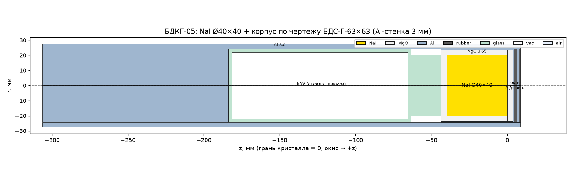
Геометрия блока БДКГ-05 построена по чертежу родственного блока детектирования с заменой кристалла на Ø40×40 мм: NaI(Tl) + отражатель MgO 3.65 мм + Al-стакан, воздушный зазор, стенка корпуса Al 3 мм, входное окно (MgO/Al/резина), ФЭУ-хвост (стекло + вакуум); полная длина 315 мм (Рис. 3). Показание моделируется как энерговыделение в кристалле с пересчётом в нЗв/ч через калибровку прибора по Cs-137.

Разрез модели блока БДКГ-05 в Geant4 — **Рис. 3.** Модель блока БДКГ-05 в Geant4: кристалл NaI(Tl) Ø40×40 мм, отражатель MgO, Al-корпус 3 мм, входное окно, ФЭУ-хвост.

Энергетическая чувствительность. Отклик на единицу H*(10) фронтального пучка имеет пик ×2.1 при 100–150 кэВ — некомпенсированный NaI (Рис. 4). Однако жёсткий спектр ДПР этим пиком практически не задевается: свёртка S(E) по полному спектру ²¹⁴Pb + ²¹⁴Bi даёт коэффициент 1.004 — прибор считывает H*(10) поля ДПР без искажения.

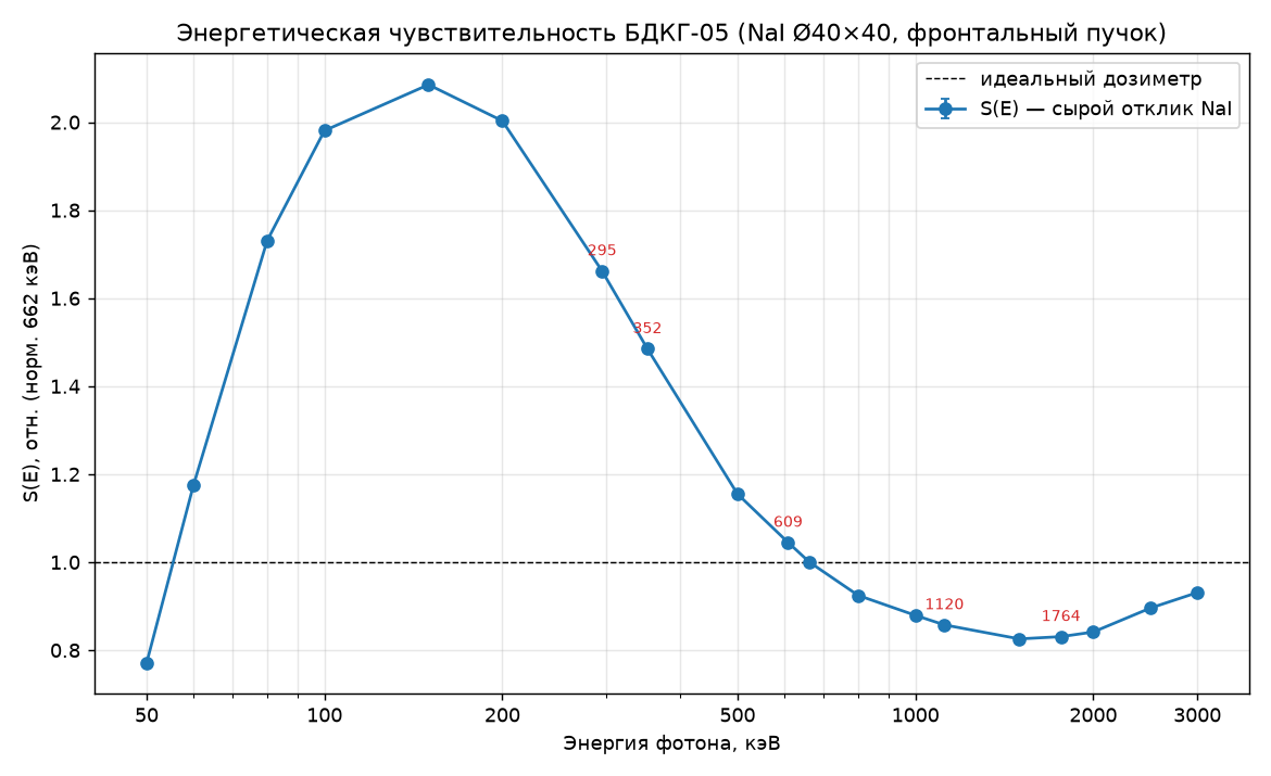
Энергетическая чувствительность БДКГ-05 на единицу H*(10) — **Рис. 4.** Энергетическая чувствительность S(E) на единицу H*(10) (нормировка на 662 кэВ). Красным отмечены главные линии ДПР — они лежат в области, где отклик близок к единице; свёртка по полному спектру ДПР — 1.004.

Кривая S(E) получена расчётом при нормальном падении — стандартная реперная геометрия характеристики чувствительности, в которой прибор и калибруется по Cs-137; объёмность (почти изотропность) реального поля излучения учтена отдельно — угловой свёрткой ниже, а окончательно — полной сценой §5.2–5.3, где показание 0.754 получается прямым транспортом фотонов из их реальных положений и уже содержит фактический энергетический и угловой отклик прибора (кривая S(E) на итог не умножается). Пик при 100–150 кэВ не влияет на вывод потому, что линии ДПР лежат выше 240 кэВ, где отклик плоский; форма пика при других углах падения роли не играет — линии ДПР в область этого пика не попадают.

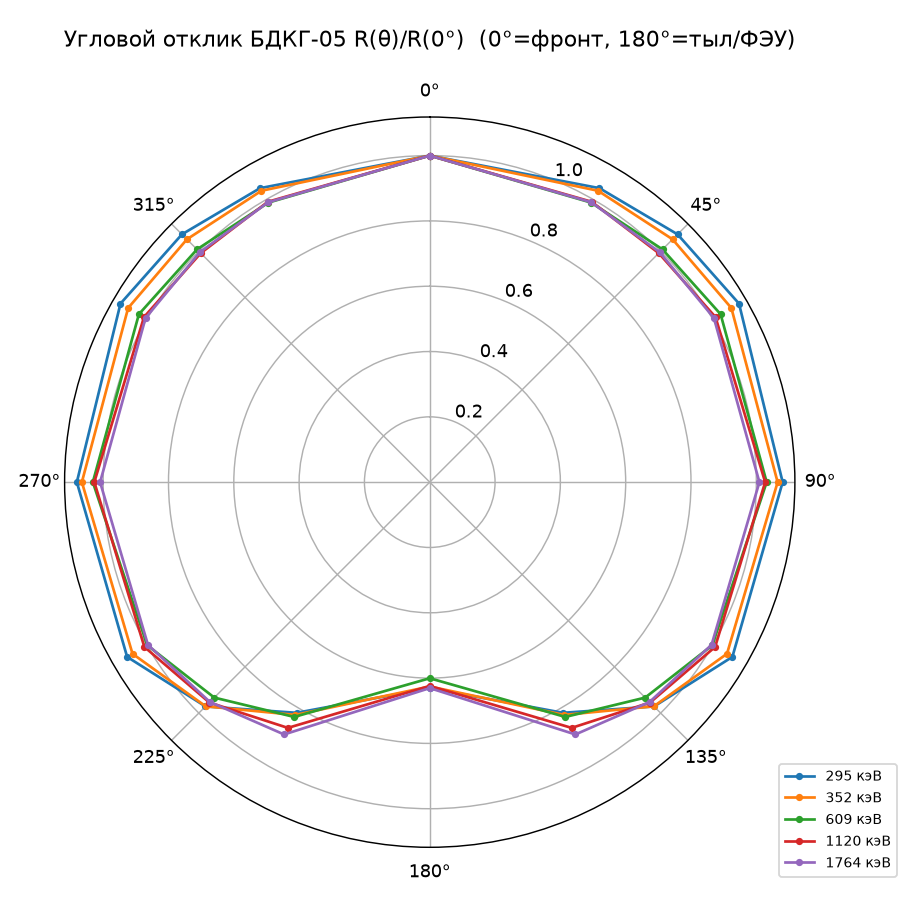
Угловой отклик. R(θ)/R(0°) на линиях ДПР 295–1764 кэВ: фронт–бок ±9 %, тыл 0.60–0.63 (экранировка ФЭУ-хвостом); свёртка по изотропному полю излучения −3…+2 % (Рис. 5). Совместно с энергетическим откликом (1.004 × (0.97…1.02) = 0.97…1.03) инструментальные отклики в изотропном поле излучения искажения не вносят — единицы процентов; паспортная оценка углового отклика (+3.5…+5.9 %, §6.3) — того же порядка.

Угловой отклик БДКГ-05 на линиях ДПР — **Рис. 5.** Угловой отклик R(θ)/R(0°) на пяти линиях ДПР (0° — фронт, 180° — тыл/ФЭУ).

5.2. Сцена и схема расчёта

Сцена — фактическая Г-комната по CAD-плану (Рис. 1): бетонные ограждения 300 мм (физический источник комптоновского рассеяния), кирпичный лестничный блок 335 мм, стальная столешница 1.5 мм, прибор в фактической позиции и ориентации. Камерная модель §3.1 реализована заново, независимым кодом, и сверена с аналитикой по контрольным точкам: коэффициент равновесия и все табличные активности воспроизведены (F = 0.567/0.677 против 0.568/0.677 аналитики). Транспорт разделён со свёрткой: Geant4 считает отклик на один фотон каждого источника (объём воздуха, пол, потолок, стены, столешница, корпус; до 5·10⁷ фотонов на прогон) по полному набору 110 линий LNHB/DDEP, а активности камерной модели прикладываются постобработкой — все чувствительности получаются из одних и тех же прогонов. Статистическая погрешность воздушных компонент 2–3 %, осаждённых — доли процента. Геометрии методов различаются в мелочах (аналитика: лестничный блок 2130 мм, V = 88.51 м³; Geant4: блок 2149 мм, V = 88.3 м³ — CAD-неувязка 19 мм): расхождение объёмов 0.2 %, пренебрежимо.

Кросс-проверка транспорта: прямая воздушная компонента приращения Ḣ*(10) — 0.3325/0.4050 (Geant4) против 0.332/0.405 (аналитика, Табл. 5) при X = 25/50 — совпадение лучше 1 % между двумя независимыми реализациями.

5.3. Показание прибора и приращение Ḣ*(10)

Таблица 7. Показание БДКГ-05 и приращение Ḣ*(10) в точке детектирования по компонентам, Geant4 (нЗв/ч на 100 Бк/м³ Rn). X — скорость присоединения ДПР к аэрозолю, мера запылённости, ч⁻¹ (§3.1); ей отвечает коэффициент равновесия F = 0.567 (X = 25) и 0.677 (X = 50). Компоненты округлены до трёх знаков; итоги — по неокруглённым значениям.
Источник	X = 25		X = 50
Источник	показание	Ḣ*(10)	показание	Ḣ*(10)
Воздух комнаты	0.419	0.382	0.509	0.465
Потолок	0.043	0.036	0.033	0.028
Пол	0.053	0.052	0.041	0.040
Стены	0.078	0.068	0.059	0.051
Столешница	0.052	0.056	0.039	0.042
Корпус прибора	0.109	—	0.083	—
ИТОГО	0.754	0.594	0.764	0.627

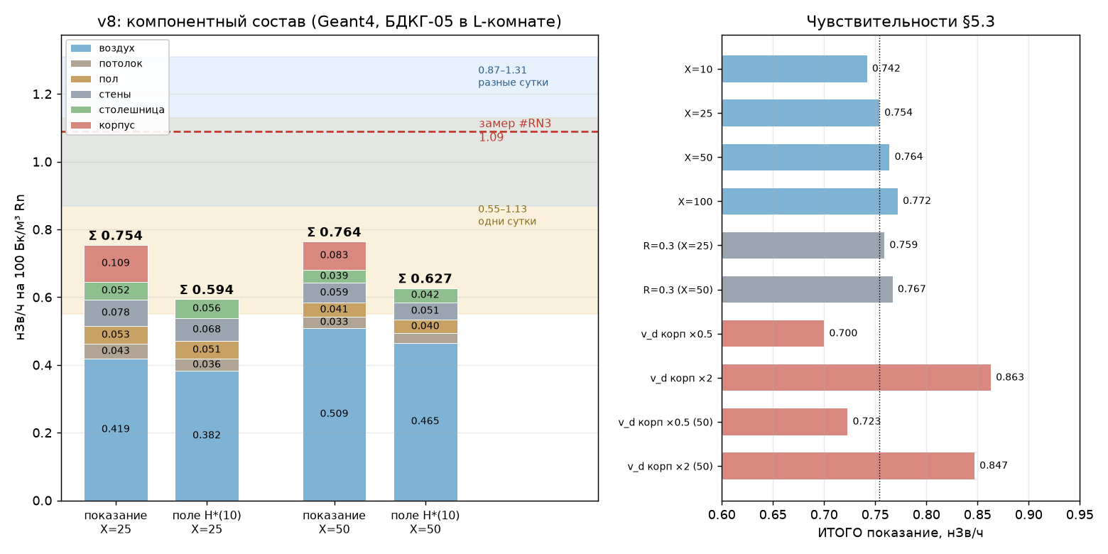
Осаждение на корпус даёт 0.083–0.109 нЗв/ч на 100 Бк/м³ — 11–14 % показания, крупнейший вклад, отсутствующий в аналитике принципиально. Вместе с близкими осаждёнными источниками (столешница, ближняя стена) он объясняет, почему показание прибора систематически выше приращения Ḣ*(10): в 1.22–1.27 раза (Рис. 6). Приращение Ḣ*(10) по Geant4 — 0.594/0.627 — согласуется с аналитикой (0.579/0.610, Табл. 5) с точностью +2.5–2.8 %; разница — итог двух встречных эффектов: физическое рассеяние больше альбедо-оценки (рассеянная доля приращения 14.5–15.1 % против +10 % модели полости — альбедо-оценка нижняя), а вклад столешницы у Geant4 меньше, что её частично компенсирует.

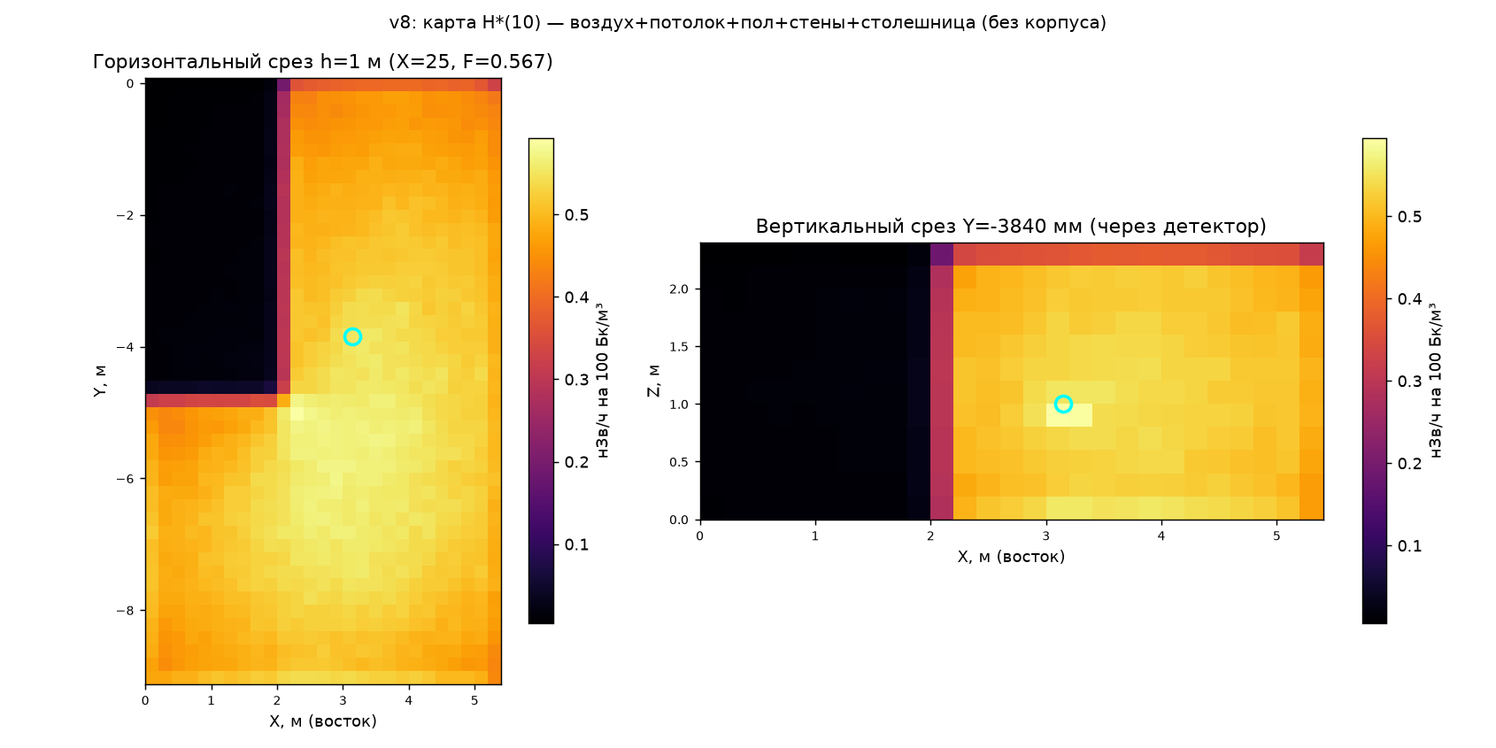
Компонентный состав показания и поля, Geant4 — **Рис. 6.** Компонентный состав показания БДКГ-05 и приращения Ḣ*(10) при X = 25/50 на фоне интервалов замера #RN3 (слева); чувствительности показания (справа).

Пространственные карты Ḣ*(10) по комнате (сетка 200 мм) подтверждают доминирование воздушной компоненты: распределение Ḣ*(10) по помещению однородно, градиенты — только у поверхностей и столешницы; карта в точке детектирования сверена с независимым сферическим оценщиком (расхождение ~1.5 %) (Рис. 7).

Карты поля H*(10) по помещению — **Рис. 7.** Карта Ḣ*(10) (без вклада корпуса): горизонтальный срез на высоте 1 м и вертикальный срез через детектор. Тёмная зона — лестничный блок.

5.4. Чувствительности показания

Все вариации — из тех же прогонов транспорта (постобработкой): запылённость X = 10/25/50/100 ч⁻¹ → показание 0.742/0.754/0.764/0.772 нЗв/ч на 100 Бк/м³ — ±2 % на декаду X: рост воздушной компоненты компенсируется падением осаждённых, включая корпус (то же свойство точки измерения, что и у аналитики, §4.4). В частности, сценарию F = 0.37–0.40 (X ≈ 10, §4.1) отвечает показание 0.742 — лишь на 2 % ниже базового. Фактор отскока R = 0.3 (согласованной парой) — +0.4…+0.6 %. Единственный значимый фактор — скорость осаждения на корпус: v_d(корпус) ×0.5 / ×2 → −5…−7 % / +11…+14 % (для стали и алюминия прямых измерений v_d нет, принято стекло как ближайший гладкий непористый материал). Пустотность плит перекрытия проверена дельта-прогоном: +0.3 %, пренебрежимо.

Интерактивное приложение. Трёхмерная модель помещения с прибором и калькулятором Ḣ*(10) по результатам этого раздела — 3D-модель помещения с калькулятором: геометрия комнаты и стенда, компоненты показания и приращения, интерактивный пересчёт под свои параметры.

5.5. Вычислительная инфраструктура и роль расчётного агента

Монте-Карло часть работы (§5) выполнена отдельным вычислительным контуром под управлением ИИ-агента (Claude Code, модель Anthropic Claude) по заданию и под контролем оператора. Организационно это ключ к независимости верификации: аналитическая линия #RN4 (§3–§4) и линия Geant4 (§5) велись как разные контуры с раздельной реализацией камерной модели и разным инструментарием — сверка шла только по контрольным точкам (§5.2), поэтому совпадение промежуточных величин (воздушная компонента приращения — лучше 1 %, коэффициент равновесия — в третьем знаке) служит доводом против общей ошибки кода. Агент самостоятельно собрал тулкит, написал геометрию, физику и скоринг на C++, управлял прогонами и выполнил свёртку и построение фигур; научные решения (входы v8, материалы, позиция прибора, разрешение разночтений спецификации) принимались оператором.

Сборка Geant4 на Windows. Использована официальная сборка CERN Geant4 11.2.1 [MT] под Windows (пакет WIN32-VC17), компилятор MSVC v143 (Build Tools 2022), система сборки CMake + Ninja; датасеты низкоэнергетической электромагнитной физики (G4EMLOW и др.) — из дистрибутива CERN. Две особенности среды потребовали обхода. Во-первых, кириллица в системных путях профиля пользователя нарушает работу инсталляторов и кэшей сборки — всё научное окружение вынесено в ASCII-пути (C:\geant4, C:\g4work, C:\g4temp). Во-вторых, в prebuilt-архиве нет import-библиотек (.lib) и Geant4Config.cmake, поэтому линковаться штатным find_package не с чем: import-библиотеки сгенерированы вручную из DLL (dumpbin /exports → .def → lib /def:), а проекты линкуются напрямую списком библиотек с определением G4LIB_BUILD_DLL. Работоспособность сборки подтверждена аналитическими проверками (флюенс точечного источника 1/4πr², массы объёмов) до постановки физических задач.

Управление прогонами. Всё управление — консольное, без GUI. Окружение поднимает один скрипт (vcvars64 + CMake/Ninja + переменные G4*DATA); каждая задача — небольшой проект main.cc + CMakeLists, параметры прогона задаются аргументами командной строки (<режим> <источник> <нуклид> <число фотонов>), физический лист — G4EmStandardPhysics_option4, порог 0.3 мм. Тяжёлые прогоны (до 5·10⁷ фотонов) шли пакетами фоновых процессов, по одному ядру на процесс; итоговые строки логов — в машинно-читаемом виде, их собирает Python-постобработка (numpy/matplotlib), где транспорт сворачивается с активностями камерной модели. Разделение «транспорт по нуклидам → свёртка с активностями постобработкой» (§5.2) — сознательное проектное решение: оно позволило получить все чувствительности §5.4 из одних и тех же прогонов, без повторного транспорта. Методическая деталь, найденная при отладке карт Ḣ*(10) (Рис. 7): трек-длинный оценщик со свободным шагом даёт ложный «горячий слой» на середине высоты (весь пролёт фотона в разреженном воздухе относится к одной ячейке середины шага); устраняется ограничением шага 100 мм (G4StepLimiter), после чего значение в точке прибора сходится с независимым сферным оценщиком в пределах ~1.5 %.

6Сравнение с экспериментом #RN3

6.1. Целевые величины и их погрешности

Эксперимент #RN3 (выключение вентиляции, рост ОА радона 318 → 1193 Бк/м³) измерил коэффициент связи мощности эквивалентной дозы (МЭД) с ОА между двумя стабильными плато — уровнем при работающей вентиляции и верхним плато после набора при выключенной: +1.09 нЗв/ч на 100 Бк/м³ (95 % ДИ 1.03–1.16)[15]. На стабильных уровнях ДПР находятся в равновесии со своей ОА, поэтому именно эта величина является измерением коэффициента; он определяется однократно за эксперимент. Регрессионные оценки по переходным данным отдельных суток отягощены малым отношением сигнал/фон и статистически ненадёжны (одна из регрессий незначима, p = 0.17); краевые эффекты нестационарности добавляют смещение уровня единиц процентов, поэтому как коэффициент они не используются.

Доверительный интервал 1.03–1.16 отражает только статистический разброс точек. Сверх него у замера есть погрешность самого прибора: по паспорту основная относительная погрешность БДКГ-05 — ±20 % (калибровка по эталону Cs-137). Она смещает все показания МЭД одним общим множителем, поэтому и коэффициент связи МЭД с ОА масштабируется целиком на те же ±20 %, независимо от статистики. С учётом ±20 % интервал суммарной неопределённости измеренного коэффициента (статистический ДИ, расширенный инструментальной погрешностью) — 0.87–1.31 нЗв/ч на 100 Бк/м³.

Отношение сигнал/фон. Полезный эффект мал на фоне полной МЭД: за время эксперимента показание БДКГ-05 менялось в пределах 69–83 нЗв/ч, то есть радоновое приращение составило до ~14 нЗв/ч (~20 % фона) в пике набора, а бо́льшую часть времени — единицы процентов. Поэтому вариации фона порядка единиц нЗв/ч (внешнее гамма-поле, приборные дрейфы) конкурируют с сигналом, и статистический ДИ занижает реальную неопределённость коэффициента.

6.2. Сопоставление

Таблица 8. Модель против натурного замера (нЗв/ч на 100 Бк/м³).
Источник	Значение	Отношение
Приращение Ḣ*(10), аналитическая модель (Табл. 5)	0.59–0.64 (центр 0.61)	—
Приращение Ḣ*(10), Geant4 (Табл. 7)	0.594–0.627	+2.5–2.8 % к аналитике (рассеяние)
Показание прибора, Geant4 (приращение + корпус + отклик)	0.754–0.764	×1.22–1.27 к приращению
Сценарий F = 0.37–0.40 (X ≈ 10): приращение (без поправки столешницы) / показание	0.53 / 0.742	−10 % / −2 %
Измеренный коэффициент, плато–плато (стат. ДИ)	1.09 (1.03–1.16)	выше показания в 1.43–1.45 раза
Измеренный коэффициент + инстр. ±20 %	0.87–1.31	показание вне интервала; нижняя граница выше расчёта в 1.14–1.15 раза

С измеренным приращением корректно сравнивать ожидаемое показание прибора — 0.754–0.764 нЗв/ч на 100 Бк/м³ (§5.3): коэффициент #RN3 получен по показаниям того же БДКГ-05, в которые входят и осаждение на корпус, и отклик прибора. Рассчитанное показание лежит вне пределов погрешности измеренного коэффициента: измеренное значение 1.09 превышает расчёт в 1.43–1.45 раза, а нижняя граница суммарного интервала 0.87 — в 1.14–1.15 раза. Физический механизм (гамма ДПР радона) подтверждён количественно: расчёт и измерение согласуются в пределах фактора 1.5 (к нижней границе интервала — в пределах 15 %); природа оставшегося расхождения — §6.4.

6.3. Анализ альтернативных механизмов

Осаждение на корпус прибора — переведено из гипотез в число: 11–14 % показания (§5.3), учтено в ожидаемом показании.
Энергетический отклик БДКГ-05 по спектру ДПР — по Монте-Карло расчёту искажения не вносит: свёртка чувствительности по полному спектру ДПР даёт 1.004 (§5.1).
Угловой отклик БДКГ-05 — паспортная Табл. Г.6 (свёртка по изотропному полю излучения +3.5 % Co-60 … +5.9 % Cs-137) и Монте-Карло (−3…+2 %, §5.1) оба дают эффект в единицы процентов и наблюдаемого расхождения не объясняют.
Рост скоростей осаждения гамма-эмиттеров (литературный разброс v_d до 2.0–3.5 м/ч против принятых 0.43–1.24 (стены/пол/потолок 0.43–0.67, стекло-прокси подставки и корпуса 1.24)[4][6]) ограничен связкой с балансом воздуха: усиленное осаждение снижает объёмную активность ²¹⁴Pb/²¹⁴Bi в воздухе и понижает F, так что приращение дозы в рамках настоящей модели остаётся несущественным.
Нулевое осаждение — сценарий не согласуется с данными: удержание наблюдаемого неравновесия одной вентиляцией потребовало бы λ_в ≈ 1.4–2.6 ч⁻¹ (F = 0.45…0.30; полный воздухообмен каждые 23–43 минуты), что не согласуется с измеренной динамикой; доза при этом снизилась бы в несколько раз.
ДПР торона (²¹²Pb, ²⁰⁸Tl 2.61 МэВ) — по прямому измерению не проявляются: аэрозольный радиометр АльфаАэро значимой ЭРОА ДПР торона в помещении не выявил.

6.4. Возможные источники остаточного расхождения

Измеренный коэффициент (1.09) превышает показание модели (0.75–0.76) в 1.43–1.45 раза; расхождение не покрывается погрешностью измерения — нижняя граница интервала (0.87) выше расчёта в 1.14–1.15 раза. Возможные вклады в это расхождение:

Скорость осаждения на корпус прибора — главная расчётная неопределённость показания: v_d для стали/алюминия прямо не измерена, вариация ×2 даёт +11…+14 % (§5.4).
Фоновая вариабельность между плато — сигнал мал относительно фона (§6.1), а сравниваемые плато разнесены во времени на сутки: изменения фона, не связанные с радоном, входят в измеренную разность напрямую.
Гамма из-под пола, коррелированная с ОА. Средний уровень подпольной гаммы (ДПР в грунте сквозь 30 см бетона, 3.3–6.9 длин пробега, с фактором накопления[14]) мал — 0.06–0.16 нЗв/ч при 20–50 кБк/м³ в грунте, и его постоянная часть в коэффициент #RN3 не входит (регрессия вычитает константу). Однако активность ДПР в грунте под зданием и ОА в комнате управляются общим фактором — динамикой грунтового газа: коррелированная с ОА часть подпольного поля регрессией не вычитается и входит в измеренный коэффициент. Величина этой вариации в работе не оценивалась.
Внешнее гамма-поле — ДПР радона в приземном воздухе и грунте вокруг здания; вымывание ДПР осадками способно менять фон на величины, сопоставимые с сигналом (§7).

7Ограничения

Изотропно перемешанный воздух, установившийся режим (переходные процессы 3–4 ч после смены вентиляции не моделируются).
Кратность воздухообмена измерена в предположении постоянного источника; суточный ход поступления грунтового газа учтён только расширением диапазона λ_в.
Коэффициент равновесия F независимо не измерялся — он вычислен моделью при нормативной запылённости (X = 25–50 ч⁻¹, сама запылённость тоже не измерялась). Сценарий по прямым измерениям F при отключённой вентиляции (0.35–0.45[21]) учтён в бюджете: −9…−12 % приращения, −2 % показания (§4.3, §5.4). Прямая проверка — одновременный замер ОА (RadonEye) и ЭРОА (АльфаАэро): F = ЭРОА/ОА.
Комптон в аналитике — модель полости с дозовым альбедо (без углового и спектрального разрешения рассеянной компоненты); альбедо выведено из первоисточников[16][18]; физический расчёт (§5.3) показывает, что это нижняя оценка (+2.5–2.8 % к приращению).
Излучение с E < 0.2 МэВ не включено (нижняя граница таблиц модели): гамма ²¹⁴Pb 53–196 кэВ и K-рентген висмута 75–90 кэВ — керма-взвешенно ≈ 2 % итога; слабые линии с выходом < 0.03 % — ещё ≈ 1 % энергии.
Скорости осаждения привязаны по типу поверхности, а не измерены для конкретных материалов; для стали подставки и корпуса прибора взяты данные стекла — ближайшего гладкого непористого материала (§2); отсюда главная чувствительность показания v_d(корпус) ×0.5/×2 → −7…+14 % (§5.4).
Геометрия блока детектирования в Geant4 — по чертежу родственного блока с заменой кристалла; внутренние узлы ФЭУ упрощены.
Торон (²²⁰Rn) и его ДПР в модель не включены (значимого вклада по замерам не выявлено, §6.3).
Инструментальная погрешность БДКГ-05 (±20 %) отнесена к целевой величине замера (суммарный интервал), не к модели.
Оценивается только приращение от ДПР радона; постоянная часть природного фона (космика, ⁴⁰K, ряды U/Th, подпольная гамма) в коэффициент #RN3 не входит. Вариации фона, коррелированные с ОА или совпавшие по времени с набором (перераспределение ДПР в грунте под зданием, внешнее гамма-поле при осадках), регрессией не вычитаются — условие корректности замера включает сухую погоду в период измерений (§6.4).
Предельная схема эксперимента, свободная от связи «источник в грунте ↔ гамма-поле из-под пола», — подача радона в комнату от удалённого источника, не влияющего на измеряемую МЭД.

8Выводы

Построена стационарная камерная модель гамма-поля ДПР радона с раздельными фракциями, нуклид- и материал-специфичным осаждением и переносом по полному набору гамма-линий LNHB/DDEP (110 линий, ≥ 99 % гамма-энергии) — по фактической Г-образной геометрии помещения (V = 88.5 м³, затенение лестничным блоком). Входные величины восстановлены из данных эксперимента: кратность воздухообмена измерена по динамике набора радона (λ_в ≈ 0.01–0.07 ч⁻¹ — почти герметичный режим), коэффициент равновесия вычислен моделью: F = 0.57–0.68 при нормативной запылённости.
Выполнена независимая численная верификация в Geant4 с полной геометрией блока детектирования и помещения. Кросс-проверка двух методов: воздушная компонента приращения совпала лучше 1 %, коэффициент равновесия — в третьем знаке. Энергетический и угловой отклик БДКГ-05 по спектру ДПР искажения не вносят (свёртка 1.004; изотропная свёртка углового отклика −3…+2 %).
Приращение Ḣ*(10): 0.59–0.64 нЗв/ч на 100 Бк/м³ (аналитика; Geant4 0.594–0.627, физическое рассеяние поднимает альбедо-оценку на +2.5–2.8 %). Доминирует воздушная компонента (63–73 % прямых); зависимость от ОА линейна. Ожидаемое показание прибора: 0.75–0.76 нЗв/ч на 100 Бк/м³ — выше приращения в 1.22–1.27 раза, главным образом за счёт осаждения ДПР на корпус (11–14 % показания).
Итог устойчив к главной неизмеренной паре «запылённость–коэффициент равновесия»: показание меняется лишь на ±2 % на декаду X; сценарию прямых измерений F = 0.35–0.45 при отключённой вентиляции отвечает показание −2 % (приращение −9…−12 %). Крупнейшая неопределённость — скорость осаждения на корпус (×0.5/×2 → −7…+14 % показания); материал подставки после пересчёта на фактической геометрии — лишь −1…−2 % поля.
Измеренный между двумя стабильными плато коэффициент — 1.09 нЗв/ч на 100 Бк/м³ (95 % ДИ 1.03–1.16); с калибровочной погрешностью БДКГ-05 ±20 % — суммарный интервал 0.87–1.31. Рассчитанное показание 0.75–0.76 лежит вне пределов погрешности измерения: измеренное значение превышает его в 1.43–1.45 раза, нижняя граница интервала — в 1.14–1.15 раза. Физический механизм — гамма ²¹⁴Pb/²¹⁴Bi — подтверждён количественно двумя независимыми реализациями: расчёт и измерение согласуются в пределах фактора 1.5; кандидаты остатка — §6.4.
Рассмотрены и признаны несущественными: энергетический и угловой отклик прибора (Geant4 + паспорт), рост скоростей осаждения гамма-эмиттеров (связка с балансом воздуха), сценарий нулевого осаждения; ДПР торона по замеру АльфаАэро не проявляются. Возможные источники остаточного расхождения: скорость осаждения на корпус, вариабельность замера при малом отношении сигнал/фон, коррелированная с ОА подпольная гамма и внешнее поле (§6.4).

9Заявление об использовании ИИ

Работа выполнена в связке «оператор + ИИ-агенты» (интерфейс Claude Code, Anthropic). Роли распределены так:

Аналитическая линия (§2–§4, §6–§8: вывод и реализация камерной модели, расчётные скрипты, обработка данных #RN3, иллюстрации, двуязычный текст статьи) — ИИ-агент Claude Code; модели Anthropic Claude Fable 5 и Claude Opus 4.8.
Монте-Карло верификация (§5) — отдельный ИИ-агент Claude Code на другой машине, с независимой реализацией камерной модели и собственным инструментарием (Geant4, C++); сверка с аналитической линией — только по контрольным точкам (§5.2, §5.5).
Аудит — третий, независимый ИИ-агент: перед публикацией каждой версии — сверка формул выводом из первых принципов, репродукция численных результатов запуском кода, сверка текста с первоисточниками; предписания аудита исполнялись до публикации.
Оператор (человек): постановка задачи, все натурные измерения (#RN3, микроклимат, торон), выбор и подтверждение входных данных (геометрия по CAD-плану, материалы, позиция прибора), приёмка каждого шага, критические замечания к формулировкам и методике, решения о публикации. Ответственность за постановку эксперимента и итоговые выводы — на операторе.
Внешний специалист (человек): независимые замечания по методике и данным — измеренный диапазон коэффициента равновесия[21], условия применимости замера; учтены в §4.1, §6.1, §6.4, §7.

Все ключевые числа воспроизводимы приложенным кодом (см. блок «Код и воспроизведение» ниже); совпадение результатов двух независимо реализованных расчётных линий (§5.2) — часть контроля качества.

10Список литературы

Jacobi W. Activity and potential alpha-energy of ²²²radon and ²²⁰radon daughters in different air atmospheres // Health Physics. — 1972. — Vol. 22, № 5. — P. 441–450. (камерная модель)
Porstendörfer J. Properties and behaviour of radon and thoron and their decay products in the air // Journal of Aerosol Science. — 1994. — Vol. 25, № 2. — P. 219–263. (разделение фракций, присоединение, осаждение)
Doses from radon progeny as a source of external beta and gamma radiation / V. M. Markovic, D. Krstic, D. Nikezic, N. Stevanovic // Radiation and Environmental Biophysics. — 2012. — Vol. 51. — P. 391–397. (ур. камерной модели; сверено по PDF)
Radon progeny surface deposition and resuspension — residential materials / B. E. Leonard [et al.] // Proceedings of the 1994 International Radon Symposium. — Atlantic City, 1994. — P. III-3. (скорости осаждения по материалам, фактор отскока; сверено по PDF)
Nazaroff W. W., Kong D., Gadgil A. J. Numerical investigations of the deposition of unattached ²¹⁸Po and ²¹²Pb from natural convection enclosure flow : preprint LBL-30249. — Berkeley : Lawrence Berkeley Laboratory, 1992. — 39 p. (ориентационная зависимость v_d; сверено по PDF)
Experimental investigation of deposition velocity of ²²²Rn progeny in a walk-in-type calibration chamber at different ²²²Rn concentrations / A. P. Vijith, R. Mishra, B. K. Sapra, Y. S. Mayya, N. Karunakara : препринт. — SSRN, 2025. — № 5610572. — (не рецензирован). (v_d ⊥ ОА, турбулентность; сверено по PDF)
Mercer T. J. The effect of particle size on the escape of recoiling RaB atoms from particulate surfaces // Health Physics. — 1976. — Vol. 31, № 2. — P. 173–174. (фактор отрыва при α-распаде; значение 0.83 цитировано по [4], стр. 7)
Источники и эффекты ионизирующего излучения : отчёт НКДАР ООН 2000 г. Генеральной Ассамблее. Т. I: Источники. Приложение B. — Нью-Йорк : ООН, 2000. (веса ЭРОА, p. 103, § 122)
ГОСТ Р ИСО 4037-3–2019 (ISO 4037-3:2019). Защита радиационная. Эталонное рентгеновское и гамма-излучение … Часть 3. — Введ. 2019. (h*_K(E): керма → H*(10))
Hubbell J. H., Seltzer S. M. Tables of X-ray mass attenuation coefficients and mass energy-absorption coefficients : NIST Standard Reference Database 126. — Gaithersburg : NIST, 1995. (μ/ρ, μ_en/ρ воздуха)
Chisté V., Bé M.-M. ²¹⁴Pb, ²¹⁴Bi — Table de Radionucléides / LNE–LNHB/CEA (Decay Data Evaluation Project). — Saclay, 2007–2010. (энергии и выходы гамма-линий и рентгена; сверено по PDF, контрольные суммы Σ E·y совпали)
Conversion coefficients for use in radiological protection against external radiation : ICRP Publication 74 // Annals of the ICRP. — 1996. — Vol. 26, № 3–4. (коэффициенты перехода к H*(10))
Cember H., Johnson T. E. Introduction to Health Physics. — 4th ed. — New York : McGraw-Hill, 2009. (ядро точечного источника exp(−μr)/4πr²)
Trubey D. K. New gamma-ray buildup factor data for point kernel calculations : ANS-6.4.3 : ORNL/RSIC-49. — Oak Ridge : ORNL, 1988. (факторы накопления бетона; значения — оценка, требуют сверки)
Отчёт по эксперименту #RN3 «БДКГ-05 ↔ RadonEye», контур «Радоновый риск». — 12.07.2026. (целевые величины; паспорт БДКГ-05: осн. погрешность ±20 %)
Chilton A. B., Huddleston C. M. A semiempirical formula for differential dose albedo for gamma rays on concrete // Nuclear Science and Engineering. — 1963. — Vol. 17, № 3. — P. 419–424. (дифференциальное дозовое альбедо бетона)
Huddleston C. M., Wilcoxson W. L. Gamma-ray streaming through ducts : Technical Report DASA 11.026 / U.S. NCEL. — Port Hueneme, 1964. — (DTIC AD 430603). (обзор альбедо; PDF сверен)
Huddleston C. M., Shoemaker N. F. Monte Carlo calculations of gamma-ray albedo : Technical Note N-764 (DASA 11.058) / U.S. NCEL. — Port Hueneme, 1965. — (DTIC AD 0621441). (параметры C, C′; PDF сверен — источник a_D(E))
Geant4 — a simulation toolkit / S. Agostinelli [et al.] // Nuclear Instruments and Methods in Physics Research A. — 2003. — Vol. 506, № 3. — P. 250–303. (инструментарий Монте-Карло, §5)
Recent developments in Geant4 / J. Allison [et al.] // Nuclear Instruments and Methods in Physics Research A. — 2016. — Vol. 835. — P. 186–225. (современные версии тулкита)
Прямые измерения коэффициента равновесия F в помещениях при отключённой вентиляции: F = 0.35–0.45 (частное сообщение, июль 2026). (сценарий §4.1, §4.3, Табл. 6)

Статус входных данных: гамма-линии — полный набор LNHB/DDEP [11] (110 линий E ≥ 0.2 МэВ, y ≥ 0.03 %; Σ E·y = 99.5 %/99.0 % полных значений; исключённый диапазон E < 0.2 МэВ ≈ 2 % итога, §7). Веса ЭРОА — UNSCEAR 2000 Annex B, p. 103, § 122. T_½ — ENSDF/DDEP. μ/ρ, μ_en/ρ — NIST. h*_K — узлы согласованы с реперами ISO 4037-3 (0.662 МэВ → 1.21; 1.25 МэВ → 1.16 Зв/Гр). Альбедо бетона — из первоисточников [16, 18] на сетке 0.2–2.5 МэВ. Геометрия стенда — по фото; столешница — сталь 1.5 мм. λ_в — измерена по динамике набора (§3.4). Погрешность прибора — ±20 % (паспорт БДКГ-05), отнесена к суммарному интервалу замера. Формулы (1)–(5) сверены независимым выводом из первых принципов; вычисления верифицированы угловой квадратурой и сходимостью сеток (§3.5).

Код и воспроизведение: аналитика — scripts/analysis/rn_room_model.py + rn_v9_lroom.py + rn_v9_tables.py + rn_vent_from_rise.py + rn_tabletop_correction.py + rn_bdkg_band.py (Python 3.12 + numpy); Монте-Карло — Geant4 11.2.1 [MT], prebuilt CERN под Windows (MSVC v143, CMake + Ninja), сцена bdkg05_scene (C++), камерная модель jacobi_v8.py, свёртка postproc_v8.py (детали сборки и управления прогонами — §5.5). Постоянные распада: ²¹⁸Po 13.42 ч⁻¹, ²¹⁴Pb 1.552 ч⁻¹, ²¹⁴Bi 2.111 ч⁻¹. Скорости осаждения — references/deposition-velocities-materials.md. Журнал изменений — CHANGELOG_RN4_v9.md.

Контур «Радоновый риск» · линия #RN4 · версия 9.2 · 22 июля 2026 г.

Radon Risk contour · line #RN4 · v9.2 · 22 Jul 2026

Indoor gamma field of short-lived radon progeny: a nuclide-specific room model, Monte Carlo verification and a check against an in-situ measurement

Calculation of the H*(10) increment from ²¹⁴Pb and ²¹⁴Bi per unit radon concentration, with the input quantities recovered from the data of experiment #RN3[15] (BDKG-05), on the as-built room geometry. Analytical model and an independent Geant4 calculation: the Ḣ*(10) increment at the detection point ≈ 0.59–0.64, expected instrument reading ≈ 0.75–0.76 nSv/h per 100 Bq/m³.

The study was carried out by AI agents (Anthropic Claude) under the guidance and control of the operator; the Monte Carlo verification — by an independent AI pipeline; article versions were audited by a third AI agent. See §9 "Statement on the use of AI".

Objective: to relate the ²²²Rn activity concentration to the increment of the ambient dose equivalent rate Ḣ*(10) of short-lived progeny gamma radiation (²¹⁴Pb, ²¹⁴Bi) at the detection point, and to independently check the coefficient of experiment #RN3[15] — +1.09 nSv/h per 100 Bq/m³ (95 % confidence interval (CI) 1.03–1.16; the detector's own ±20 % error widens the interval to 0.87–1.31).

Instruments and room: a BDKG-05 scintillation detector unit (NaI(Tl) crystal Ø40×40 mm, basic error ±20 %) on a 370×420 mm steel stand (1.5 mm sheet), crystal centre 1.0 m from the wall, at a height of ~1 m; a RadonEye Plus2 radon monitor at the same level; an L-shaped basement room taken from the CAD floor plan (5.35×9.12 m envelope, a 2.13×4.84 m staircase block in the corner, height 2.3 m, V = 88.5 m³), 30-cm concrete floor slab.

Methods: a steady-state Jacobi room model with separate unattached and attached fractions and nuclide-specific deposition from the chamber measurements of Leonard (1994); the air-exchange rate is measured from the radon build-up dynamics after the ventilation was switched off (0.01–0.07 h⁻¹), the aerosol attachment rate is set by the regulatory dust level (X = 25–50 h⁻¹), and the equilibrium factor is a model output (F = 0.57–0.68); transport is direct point-kernel integration over the complete LNHB/DDEP gamma-line set (110 lines with E ≥ 0.2 MeV, ≥ 99 % of the progeny gamma energy) with Ḣ*(10) averaging over the crystal volume and shadowing by the staircase block; Compton scattering is a cavity model with the concrete dose albedo from the Chilton–Huddleston formula; shielding by the steel tabletop and deposition on its underside are included. Independent verification — a Monte Carlo model of the instrument and the room in Geant4 (§5): full detector-unit geometry, transport over the same 110 lines, progeny deposition on the instrument housing, energy and angular response.

Conclusion: the increment of the ambient dose equivalent rate Ḣ*(10) per unit radon concentration at the detection point is computed; the two independent implementations agree: 0.59–0.64 nSv/h per 100 Bq/m³ (analytical model) and 0.594–0.627 (Geant4). The expected BDKG-05 reading is higher than this increment by a factor of 1.22–1.27 — due to progeny deposition on the detector-unit housing (11–14 % of the reading) and the nearby deposited sources — and amounts to 0.75–0.76 nSv/h per 100 Bq/m³. The increment measured in experiment #RN3 — +1.09 nSv/h per 100 Bq/m³ (95 % CI 1.03–1.16; with the ±20 % instrument error, a total interval of 0.87–1.31) — exceeds the computed reading by a factor of 1.43–1.45, and the lower bound of the interval by 1.14–1.15: the discrepancy lies outside the measurement error limits, while the calculation and the measurement agree to within a factor of 1.5 (within 15 % of the lower bound of the interval). The nature of the discrepancy is examined in §6.4; the instrument response does not account for it (the convolution of the energy and angular sensitivity over the progeny spectrum is 1.004), nor does the unmeasured dust level (at an equilibrium factor of 0.37–0.40 the computed reading changes by only −2 %).

Keywords: radon, radon progeny, ²¹⁴Pb, ²¹⁴Bi, equilibrium factor, aerosol deposition, Jacobi room model, ambient dose equivalent H*(10), indoor gamma background, dose albedo, Monte Carlo, Geant4.

1Introduction

The radon-related gamma background is produced not by ²²²Rn itself (a noble gas, practically a pure alpha emitter at its own step in the chain) but by two members of its decay chain — ²¹⁴Pb (T_½ = 26.8 min) and ²¹⁴Bi (T_½ = 19.7 min), with lines from 0.24 to 2.7 MeV. The intermediate ²¹⁸Po (T_½ = 3.1 min) emits no gamma but, being deposited most intensively of the three, serves as the main "supplier" of the surface activity of the gamma emitters through in-situ decay.

Progeny removal from air proceeds through two channels with opposite dosimetric consequences: ventilation removes activity from the room, whereas deposition preserves it on the enclosing surfaces, where it continues to radiate. The balance of the two channels sets the equilibrium factor F ∈ (0, 1) and the split of the dose between the airborne and surface components.

The aim of this work is an independent check of the coefficient measured in experiment #RN3: an increment of the ambient dose equivalent rate of +1.09 nSv/h per 100 Bq/m³ (95 % CI 1.03–1.16; on top of the statistics — the detector's own ±20 % error, total interval 0.87–1.31, §6.1) after the basement ventilation was switched off[15]. A first-principles computational model is built: the progeny balance in air and on surfaces → source activities → gamma transport to the detector → H*(10). The input quantities are, wherever possible, recovered from the experiment's own data: the air-exchange rate is measured from the radon build-up dynamics, the room geometry is taken from the building CAD plan, the stand geometry from a photograph, the stand material is as-built (1.5 mm steel); the equilibrium factor thereby becomes a model output rather than an assumption.

The check is performed by two independent implementations: the analytical model (room balance + direct point-kernel integration, §3–§4) and a Monte Carlo calculation in Geant4[19] with the full geometry of the detector unit and the room (§5). The second method additionally answers questions fundamentally inaccessible to the analytical model: the contribution of progeny deposition on the housing of the instrument itself, and possible distortion of its energy and angular response over the progeny spectrum.

The exposition proceeds from the input data (§2) through the room model and transport (§3) to the analytical results (§4), the Monte Carlo model of the instrument (§5) and the check against the in-situ measurement (§6).

2Input data

Room. An L-shaped basement room taken from the building CAD plan (internal dimensions): a 5.35 × 9.12 m envelope with a 2.13 × 4.84 m staircase block in the corner, height 2.3 m; V = 88.5 m³, floor/ceiling area 38.5 m² each, walls 66.6 m² (S/V = 1.62 m⁻¹). Construction: the staircase-block wall is 335 mm brick, the other walls are precast concrete blocks, all plastered and covered with non-woven wallpaper; ceiling — concrete slab; floor — parquet board over a 30-cm concrete slab. The brick staircase wall (~4.7 mean free paths at 0.6 MeV) is opaque to gamma radiation: the part of the room behind it is shadowed and excluded from transport.

Plan of the L-shaped basement room with the BDKG-05 detector position — **Fig. 1.** Room plan from the basement CAD drawing: 5.35 × 9.12 m envelope, staircase block (hatched) 2.13 × 4.84 m in the north-west corner. The BDKG-05 detector is 1.0 m from the staircase-block wall and 1.0 m from its end, front facing east. *(Figure labels are in Russian.)*

Setup. The detector — a BDKG-05 scintillation unit (NaI(Tl) crystal Ø40×40 mm) on a 370 × 420 mm steel stand (1.5 mm sheet): the crystal centre is 1.0 m from the staircase-block wall and 1.0 m from its southern end (Fig. 1), at a height of ≈ 1 m, axis horizontal (east–west, the PMT tail towards the wall), 3 cm above the tabletop. The RadonEye Plus2 radon monitor is at the same level.

Input quantities. The air-exchange rate is measured from the radon build-up dynamics after the ventilation was switched off (method — §3.4): λ_v ≈ 0.01–0.07 h⁻¹, adopted 0.02 h⁻¹ — the room is nearly airtight in this state. The aerosol loading is set at the regulatory level: the PM2.5 limit (0.035 mg/m³ daily average) corresponds, for the ~0.2 μm accumulation mode, to a number concentration of ~5×10³–10⁴ cm⁻³, i.e. a progeny attachment rate X ≈ 25–50 h⁻¹[2]. Deposition velocities are direct chamber measurements of seven residential materials, normalized to a standard room[4] (v_d = λ_dep·V/S, m/h):

Table 1. Progeny deposition velocities and equilibrium factor by material (Leonard 1994).
Material	`v`(²¹⁸Po)	`v`(²¹⁴Pb)	`v`(²¹⁴Bi)	F
Concrete	4.6	0.43	0.04	0.50
Wood (lacquered)	5.2	0.60	0.04	0.47
Glass	5.7	1.24	0.08	0.41
Wallboard	6.2	0.67	0.03	0.43
Ceiling tile (rough)	8.9	0.58	0.05	0.32
Carpet	9.2	2.04	0.10	0.33
Drape	17.0	3.59	0.16	0.22

Mapping to the geometry: the effective deposition surface is the one in contact with the air, not the structural material behind it — ceiling — concrete, walls — wallboard (the smooth paper surface of the non-woven wallpaper), floor — lacquered wood, stand — glass as the closest smooth non-porous material (no direct data exist for steel; metal, being a conductor, holds no static charge, so there is no electrostatic deposition component). For Compton scattering, by contrast, wallpaper and plaster are radiation-transparent — the substrate (brick/concrete) does the scattering, so the concrete albedo is used. Nuclear data: the complete LNHB/DDEP gamma-line set[11] — 110 lines with E ≥ 0.2 MeV and yields ≥ 0.03 % (16 lines of ²¹⁴Pb + 94 lines of ²¹⁴Bi), covering 99.5 % and 99.0 % of the nuclides' gamma energy (Σ E·y = 0.2217 of 0.2228 and 1.4532 of 1.4678 MeV/decay); air μ/ρ and μ_en/ρ — NIST[10]; air kerma → H*(10) conversion — h*_K(E)[9][12].

3Methods

The calculation is split into three independently controlled steps: the balance of progeny activities in air and on the surfaces (§3.1–§3.2), radiation transport to the detection point (§3.3), and the dosimetric folding; each step enters the total linearly, computational control — §3.5.

3.1. Room model of the progeny

The room is treated as a single well-mixed chamber (the Jacobi model[1]; the formulation with fractions — Porstendörfer[2]). The steady-state balance of each chain member:

(1)0 = λ_i·C_i−1 − (λ_i + λ_v + λ_dep,i)·C_i

The parent-decay input is written as λ_i·C_i−1 — with the decay constant of the daughter nuclide: C_i−1 (the parent activity) equals the birth rate of daughter atoms, and multiplying by λ_i converts the atom balance into an activity balance.

Symbols of equation (1). Physical meaning: production from parent decay = total removal (decay + ventilation + deposition).
Symbol	Quantity	Unit	Value / relation
`i`	decay-chain member index	—	1 → ²¹⁸Po, 2 → ²¹⁴Pb, 3 → ²¹⁴Bi; parent i−1 = 0 → ²²²Rn
`C`_i	airborne activity concentration of the i-th progeny	Bq/m³	sought
λ_i	decay constant of the i-th nuclide	h⁻¹	= ln2/T_½; Po 13.42, Pb 1.552, Bi 2.111
λ_v	air-exchange rate	h⁻¹	measured: 0.01–0.07; adopted 0.02 (§3.4)
λ_dep,i	effective deposition rate of the i-th nuclide	h⁻¹	= Σ_s v_d,i,s·A_s/V (Table 1)

The primary model is the full one, with separate unattached and attached fractions of each progeny: attachment to the aerosol at a rate X, ²¹⁴Pb detachment at the alpha decay of attached ²¹⁸Po (p = 0.83[7]), nuclide- and material-specific deposition of the unattached fraction (Table 1), diffusive deposition of the attached one (0.1 m/h[2]) and a vertical gravitational settling term ±v_s (v_s = 0.012 m/h for AMD ≈ 200 nm; floor/stand +, ceiling −). The equilibrium factor is then a model output:

(2)F = 0.105·f₁ + 0.515·f₂ + 0.380·f₃, f_i = C_i/C₀

where f_i is the activity fraction of the i-th progeny (the sum of both fractions) relative to the radon concentration C₀; 0.105, 0.515, 0.380 — the EEC weight factors, the shares of potential alpha energy carried by ²¹⁸Po, ²¹⁴Pb, ²¹⁴Bi (UNSCEAR 2000 Annex B, p. 103, § 122[8]).

For the lower-bounding scenarios a single-group approximation is used (one effective λ_dep,i per nuclide, no fraction split): F is fixed (0.3 or 0.4) and λ_v is recovered by inversion of (2). The single-group approximation deviates from the full model by a few per cent (§4.4).

3.2. Surface activity

The activity of each link on a surface follows from the steady-state balance "deposition from air + ingrowth from the deposited parent = decay". The key mechanism is the decay of deposited ²¹⁸Po directly on the surface; a fraction of the newborn ²¹⁴Pb is lost to recoil resuspension (factor R[4]):

(3)A_Po = v_PoC_Po/λ_Po; A_Pb = v_PbC_Pb/λ_Pb + (1−R)·A_Po; A_Bi = v_BiC_Bi/λ_Bi + A_Pb

Derivation. Steady state of atoms on the surface: λ_dau·N_dau = v_d·n_air + (1−R)·λ_par·N_par, where n_air = C/λ_dau is the atom concentration in air and λ_par·N_par = A_par. The left-hand side is A_dau itself, whence (3). Control: at R = 0 and v_Pb = v_Bi = 0 the formula must yield secular equilibrium A_Po = A_Pb = A_Bi — the test is built into the script (PASS). In the full model the surface influx sums both fractions.

where A_i are the surface activities, Bq/m²; v_i are the deposition velocities onto the given surface, m/h (Table 1); C_i are the airborne concentrations, Bq/m³; and R is the recoil-resuspension factor. R = 0.5 is adopted — the computational column of the source's Table 1[4] (the theoretical maximum for a plane); measured values for the room materials are 0.29–0.36, concrete unmeasured (extrapolation ~0.30). Importantly, the v_d(²¹⁴Pb) of Table 1 were computed by the authors assuming R = 0.5, so R can only be varied as a consistent pair (R, v_d(Pb|R)): v_Pb(R) = v_Pb(0.5) − (0.5−R)·(v_Po/λ_Po)·(λ_Pb + v_Pb(0.5)/0.6818); control point — concrete: R = 0.3 → v_d(Pb) = 0.28 m/h. The ingrowth and direct-deposition effects are then opposed and almost fully compensate: over the whole range R = 0.29–0.55 the total changes by only ±0.5 % (§4.4).

Jacobi deposition ≠ gravitational settling. "Deposition" (λ_dep) is the progeny flux to surfaces through the near-surface boundary layer, driven by diffusion (Brownian + turbulent), not by gravity; it is isotropic and governed by the fast unattached fraction (~1 nm, v_d ≈ 5–20 m/h). Bulk transport is provided by convection (5–20 cm/s, a room turnover in tens of seconds); the limiting step is the last millimetre-scale boundary layer: δ = D/v_d ≈ 4 mm; pure molecular diffusion would carry an atom only √(6Dτ) ≈ 9 cm during its lifetime. Gravitational settling is a separate vertical mechanism (v_s ≈ 0.01 m/h, attached fraction only, horizontal surfaces only) and is negligible in the total (< 0.5 %); the real orientational asymmetry comes from natural convection — vertical walls deposit ≈ 1.8× more strongly than horizontals[5].

3.3. Transport and dosimetry

The fluence at the detector is computed by direct integration of the point isotropic source kernel with exponential attenuation in air[13], separately for three sources (the air volume, the room faces, the stand), each with its own activity:

(4)G_vol(E) = ∫_V e^−μr/(4πr²) dV, G_surf(E) = ∫_S e^−μr/(4πr²) dA

(5)ΔḢ*(10) = Σ_nucl Σ_lines A·y·G(E)·E·(μ_en/ρ)(E)·h*_K(E)

where G(E) are the geometric factors of the volumetric (m) and surface (dimensionless) sources; μ(E) is the linear attenuation coefficient of air, m⁻¹; r is the distance from a source element to the calculation point; A is the volumetric (Bq/m³) or surface (Bq/m²) activity; y is the line yield (photons per decay)[11]; (μ_en/ρ) is the mass energy-absorption coefficient of air[10]; and h*_K(E) is the air kerma → H*(10) conversion[9][12]. Dimensional factors omitted.

Source model. (1) Volumetric — ²¹⁴Pb/²¹⁴Bi activities uniform over the whole L-room volume, detector inside. (2) Surface — the floor, the ceiling and six wall segments (Fig. 1), each with its own activity per (3) (material and orientation differ), grouped as "ceiling / floor / walls". (3) Local — the 370×420 mm tabletop with its top-surface activity; a source centimetres from the crystal.

Numerical integration. Volume — a 5 cm grid, layer by layer; the kernel singularity at r → 0 is handled analytically: the 15 cm neighbourhood of the detector is integrated as a uniform sphere, (1 − e^−μR)/μ. Faces — a 5 cm grid (minimum r = 1.00 m — to the staircase-block wall, no singularity; deposited activity is an isotropic emitter per unit area, no cosine factors). Shadowing: volume and face elements without line of sight from the detector (behind the brick staircase wall) are excluded; the end face of the block faces away from the detector and contributes nothing. Per-face factors at 0.609 MeV: floor 0.519, ceiling 0.418, walls in total 0.547, of which the staircase-block wall (1.0 m from the detector) 0.299 — 55 % of the wall contribution, the east wall 0.169 — 31 %; in the infinite-plane limit the distance dependence is only logarithmic, (S_A/2)·E₁(μd), hence the weak sensitivity of the total to the exact detector–wall gap. Stand — a 5 mm grid; Ḣ*(10) is averaged over the crystal volume (4 mm grid, ~800 points inside the cylinder): in the near zone the point approximation makes a noticeable error.

Compton scattering — the cavity model. Air weakly attenuates the radiation (mean free path ~80 m); an unabsorbed photon reaches the envelope, a fraction a_D is reflected and irradiates the room again; the reflection series gives the cavity factor B(E) = 1/(1 − a_D(E)), multiplying the dose of each line. The integral dose albedo of concrete a_D(E) is derived from the primary source: the Chilton–Huddleston formula[16] with the C, C′ parameters of the MC fit for a thick concrete slab (Table I[18]; review[17]) is numerically integrated over the reflection hemisphere, separately for normal incidence (lower estimate) and isotropic wall irradiation (central); control: a_D(0.662 MeV, 0°) = 0.063 vs the literature 0.06–0.08. The correction amounts to +6 % (normal) … +10 % (isotropic). Limitations: the scattered addition is position-independent (the detector position enters only the direct component), the reflection series is an integrating-sphere heuristic; a fuller treatment is possible by Monte Carlo (as in[3]).

The steel tabletop (1.5 mm). 43 % of the directions reach the crystal through the tabletop — 35 % of the air geometric factor and the entire floor contribution; the steel sheet reduces this from-below flux by 0.020 nSv/h per 100 Bq/m³ (computed over all 110 lines with slant thicknesses, NIST iron data). At the same time the tabletop's underside is a deposition surface ~4.5 cm from the crystal shining through the same steel: +0.035…+0.045 nSv/h per 100 Bq/m³ (the activity of the lower plane is taken as for the ceiling — the same downward-facing orientation). The net correction of +0.013…+0.028 nSv/h per 100 Bq/m³ enters the base estimate.

3.4. Measuring the air-exchange rate

The radon build-up curve of experiment #RN3[15] allows λ_v to be determined. The radon balance in the well-mixed room air is the input from a constant source S (soil-gas entry) minus removal through two channels, ventilation and radioactive decay:

dC/dt = S − (λ_v + λ_Rn)·C(6)

For a constant S the concentration approaches balance exponentially:

C(t) = C_∞ + (C₀ − C_∞)·e^{−k t}, k = λ_v + λ_Rn, C_∞ = S/(λ_v + λ_Rn)(7)

The radon decay constant is known exactly (λ_Rn = ln2/T_½ = 0.00755 h⁻¹), so the measured "curvature rate" k gives the ventilation directly: λ_v = k − λ_Rn. The fit is three-parameter: for each trial k a linear least-squares over the basis {1, e^{−k t}} yields C_∞ and C₀, and the k with the smallest residual is chosen; the 95 % interval comes from the residual profile.

Radon build-up curve of #RN3 after ventilation shutdown with two fits — **Fig. 2.** Build-up of ²²²Rn after the ventilation was switched off (RadonEye Plus2, #RN3). Before the experiment (0–20 h) the diurnal source variation is visible with the ventilation running. From 01:00 on 12 Jul (x = 22 h) — an almost linear rise of ~65 Bq/m³·h over 14 h with no flattening. The abrupt plateau at ~1230 Bq/m³ from 16:00 is a diurnal decrease of soil-gas entry, not a ventilation balance. The lines are the fit of Eq. (7) over two windows. *(Figure labels are in Russian.)*

The almost linear rise for 14 hours with no flattening is the signature of a nearly airtight room: the time constant τ = 1/k is large compared with the observation window, so only the early, weakly curved part of the exponential is seen. The fit result depends on whether the plateau is included:

Fit of the build-up curve over two windows (λ_Rn = 0.00755 h⁻¹).
Fit window	Points	k, h⁻¹	C_∞, Bq/m³	λ_v = k − λ_Rn, h⁻¹
Pure rise (22–36 h)	79	0.020	3504 (unphysical)	0.012 [0.012–0.021]
With plateau (22–43 h)	118	0.064	1638	0.056 [0.043–0.070]

In the pure-rise window the curve is almost straight and the asymptote is undetermined — extrapolation gives an unphysically high C_∞ ≈ 3500 Bq/m³; the window reliably shows only that λ_v is small (≲ 0.02 h⁻¹). In the window with the plateau the formal fit explains the flattening as a ventilation balance and raises λ_v to 0.056, but the plateau sets in abruptly (~1 h) and exactly at the diurnal maximum — this is a source decrease, not a smooth exponential saturation (the same diurnal variation is seen before the experiment too), so 0.056 is an upper bound. The final estimate is λ_v ≈ 0.01–0.07 h⁻¹, physically a nearly airtight room (λ_v ≲ 0.05); the ~30-min RadonEye lag is negligible on the 14-hour scale. The calculations adopt λ_v = 0.02 h⁻¹; the sensitivity of the total to the 0.01–0.05 range is +0.8…−2.3 % (§4.4), because at such weak air exchange the progeny balance is set by deposition, not ventilation. It also follows that the observed disequilibrium cannot be attributed to ventilation alone, without deposition: that would require λ_v ≈ 1.4–2.6 h⁻¹ (§6.3).

3.5. Verification of the computations

The computational script includes mandatory checks: the secular-equilibrium test for (3) (at R = 0 and zero direct deposition A_Po = A_Pb = A_Bi; failure aborts the run) and residual control |F − F_target| after bisection in the solvers. The air component is additionally verified by an independent angular quadrature (1.28×10⁶ rays, the radial integral analytic — no singularity at all): agreement with the grid method +0.4 %. Mesh convergence: halving the step changes the face factors in the 5th digit and the stand factor by 0.04 %. Linearity of the dose in the radon concentration is exact algebraically and confirmed experimentally (v_d independent of concentration[6]).

4Results

4.1. The equilibrium factor as a model output

At the measured ventilation the equilibrium factor is set by the aerosol loading — the progeny-to-aerosol attachment rate X (§3.1):

Table 2. Equilibrium factor and unattached ²¹⁸Po fraction vs aerosol loading (λ_v = 0.02 h⁻¹).
X (attachment rate), h⁻¹	Dust level	F (output)	Unattached ²¹⁸Po fraction
5	very clean air	0.30	0.73
10	clean air	0.41	0.58
25	≈ PM2.5 limit	0.57	0.35
50	typical dwelling	0.68	0.21
100	dusty	0.76	0.12

The base range X = 25–50 gives F = 0.57–0.68 (EEC 57–68 Bq/m³ per 100 Bq/m³). The dust level in the room was not measured, so F here is a computed quantity for the regulatory aerosol. Direct measurements of the equilibrium factor in rooms with the ventilation switched off give F = 0.35–0.45[21]; within the model, at the measured λ_v = 0.02 h⁻¹, such values correspond to clean air (X ≈ 8–10 h⁻¹) and are treated as a separate scenario (§4.3, §4.4). Reaching F ≤ 0.45 by ventilation at the regulatory aerosol is impossible — it would require λ_v ≈ 0.7–1 h⁻¹, excluded by the measured build-up dynamics (§3.4).

4.2. Activities in air and on surfaces

Table 3. Airborne progeny activity (Bq/m³ per 100 Bq/m³ Rn; sum of the unattached and attached fractions). X is the progeny-to-aerosol attachment rate, h⁻¹ (§3.1): 25 — the regulatory dust level, 50 — a typical dwelling.
Nuclide	X = 25	X = 50
²¹⁸Po	80.4	86.7
²¹⁴Pb	56.2	67.9
²¹⁴Bi	51.0	62.3

Table 4. Surface activity of ²¹⁴Pb / ²¹⁴Bi (Bq/m² per 100 Bq/m³ Rn). X is the aerosol attachment rate, h⁻¹ (§3.1).
Surface	X = 25		X = 50
Surface	²¹⁴Pb	²¹⁴Bi	²¹⁴Pb	²¹⁴Bi
Ceiling (concrete)	19.2	21.7	14.1	16.9
Walls (wallpaper)	25.5	28.4	18.4	21.5
Floor (parquet)	22.2	25.4	16.6	20.1
Stand (steel)	23.1	26.3	17.1	20.6

Higher aerosol loading shifts activity from the surfaces into the air: the aerosol intercepts ²¹⁸Po before deposition (unattached fraction 0.35 → 0.21), the surface ingrowth fades, the airborne ²¹⁴Pb/²¹⁴Bi grow. At the measurement point these shifts almost compensate in the dose (§4.4).

4.3. Dose rate

Table 5. Component-wise increment ΔḢ*(10) and the base estimate (nSv/h per 100 Bq/m³ Rn). X is the aerosol attachment rate, h⁻¹ (§3.1).
Component	X = 25	X = 50
Room air	0.332	0.405
Ceiling (concrete)	0.027	0.021
Walls (wallpaper)	0.047	0.035
Floor (parquet)	0.040	0.031
Stand (steel, top)	0.081	0.063
Uncollided photons, total	0.527	0.555
+ Compton (isotropic albedo)	0.579	0.610
+ tabletop (shielding −0.020; underside +0.035…+0.045)	+0.015…+0.025	+0.015…+0.025
Base estimate of the Ḣ*(10) increment	0.59–0.60	0.63–0.64

Base estimate of the Ḣ*(10) increment: 0.59–0.64 nSv/h per 100 Bq/m³, central value ≈ 0.61. At high equilibrium the air component dominates (63–73 % of the uncollided total); the stand is the largest single surface source (a large solid angle immediately adjacent to the crystal). This is an estimate of the Ḣ*(10) increment — without the instrumental effects of the detector itself (deposition on the housing, §5); the cavity albedo model is a lower estimate of scattering: the physical Compton calculation raises the field by +2.5–2.8 % (§5.3).

The F = 0.37–0.40 scenario (clean air). Direct measurements of the equilibrium factor with the ventilation off (F = 0.35–0.45) correspond in the model to X ≈ 8–10 h⁻¹: an increment of 0.52–0.53 nSv/h per 100 Bq/m³, i.e. only 9–12 % below the base — the loss of the air component (0.37 → 0.22–0.24, albedo included) is almost compensated by the growth of the surface one (0.21 → 0.29–0.31): the progeny, finding no aerosol, deposit on the walls and the stand around the detector and keep radiating. The instrument reading changes even less — by −2 % (§5.4).

4.4. Uncertainty budget

Table 6. Sensitivity of the base Ḣ*(10)-increment estimate to inputs and approximations (relative to ≈ 0.61).
Factor	Effect	Comment
The F = 0.37–0.40 scenario (X = 8–10, clean air)	−9…−12 %	largest increment uncertainty; per direct F measurements with ventilation off[21]; instrument reading −2 % (§5.4)
Wallpaper electrostatics: hypothetical v_d(walls) ×2 / ×3	−9.2 % / −16.6 %	computed hypothetical case; at the actual T ≈ 24 °C, RH 52–55 % the charge drains (humidity conductance + air ionisation) — the effect is suppressed, expected contribution 0…−3 %
Albedo variant (normal instead of isotropic)	−4 %	lower Compton estimate
Physical Compton (Geant4) instead of the albedo model	+2.5…+2.8 %	scattered fraction of the increment 14.5–15.1 % (§5.3)
Aerosol loading X = 25 ↔ 50	−3…+2 %	air ↔ surface compensation at the measurement point
Air-exchange rate 0.01 ↔ 0.05 h⁻¹	+0.8…−2.3 %	measured range
Stand material in deposition (glass → concrete)	−1…−2 %	recomputed on the L-geometry with the full fraction model; no direct data for steel
Floor: parquet ↔ concrete (deposition material)	+0.5 %	parquet board lies over the concrete slab
Tabletop correction (net range)	±1 %	+0.015…+0.025 nSv/h per 100 Bq/m³
Surface orientation (convection)[5]	−7…0 %	protocol-dependent, unstable sign; estimated on the v8 rectangular geometry
Recoil factor R = 0.29–0.55 (consistent with v_d(Pb\|R))	±0.5 %	channels compensate (§3.2)
Truncating the spectrum to the 11 main lines	−26 %	not allowed: the complete set (110 lines) is included; a spectrum property, estimated on the v8 geometry
Gravitational aerosol settling	< 0.5 %	negligible; estimated on the v8 geometry

Position-dependence caveat. The weak sensitivity to aerosol loading is a property of the measurement point (the detector next to the stand and the wall sees the airborne and surface "tiers" with comparable weight), not of the room: at the room centre the airborne share is 63–89 % and a tenfold increase of X changes the dose by +37 %.

5Numerical verification: a Monte Carlo model of the instrument and the room (Geant4)

The analytical model of §3–§4 computes the Ḣ*(10) increment at the detection point but does not answer two questions about the instrument itself: how much progeny deposition on its housing (a near source immediately adjacent to the crystal) adds to the reading, and whether the NaI(Tl) energy and angular response distorts the reading over the progeny spectrum. Both require photon transport through the real geometry of the detector unit — they are solved by Monte Carlo in Geant4 11.2[19][20] (high-precision electromagnetic physics option4, 0.3 mm cut) as an independent verification: a separate implementation of the room model, separate tooling, cross-checked against the analytical model only at control points.

5.1. Instrument model and instrumental response

The BDKG-05 geometry is built from the drawing of a related detector unit with the crystal replaced by Ø40×40 mm: NaI(Tl) + 3.65 mm MgO reflector + Al cup, air gap, 3 mm Al housing wall, entrance window (MgO/Al/rubber), PMT tail (glass + vacuum); full length 315 mm (Fig. 3). The reading is modelled as the energy deposit in the crystal, converted to nSv/h through the instrument's Cs-137 calibration.

Cross-section of the BDKG-05 unit model in Geant4 — **Fig. 3.** The BDKG-05 unit in Geant4: NaI(Tl) crystal Ø40×40 mm, MgO reflector, 3 mm Al housing, entrance window, PMT tail. *(Figure labels are in Russian.)*

Energy response. The response per unit H*(10) of a frontal beam peaks at a factor of 2.1 around 100–150 keV — uncompensated NaI (Fig. 4). The hard progeny spectrum, however, barely touches this peak: convolving S(E) with the full ²¹⁴Pb + ²¹⁴Bi spectrum gives a factor of 1.004 — the instrument reads the progeny H*(10) field without distortion.

BDKG-05 energy response per unit H*(10) — **Fig. 4.** Energy response S(E) per unit H*(10) (normalised at 662 keV). The main progeny lines (marked red) lie where the response is close to unity; the convolution over the full progeny spectrum is 1.004. *(Figure labels are in Russian.)*

The S(E) curve is taken at normal incidence — the standard reference geometry of a sensitivity characteristic, in which the instrument is also calibrated against Cs-137; the volumetric (near-isotropic) nature of the real radiation field is accounted for separately — by the angular convolution below, and definitively by the full scene of §5.2–5.3, where the reading of 0.754 is obtained by direct transport of photons from their actual positions and already contains the actual energy and angular response of the instrument (the S(E) curve is not applied to the total). The 100–150 keV peak does not affect the conclusion because the progeny lines lie above 240 keV, where the response is flat; the shape of the peak at other incidence angles is irrelevant — it is unpopulated in the hard spectrum.

Angular response. R(θ)/R(0°) at the progeny lines 295–1764 keV: front-to-side ±9 %, rear 0.60–0.63 (PMT-tail shielding); the isotropic radiation-field convolution is −3…+2 % (Fig. 5). Together with the energy response (1.004 × (0.97…1.02) = 0.97…1.03) the instrumental responses introduce no distortion beyond a few per cent in an isotropic radiation field; the datasheet estimate of the angular response (+3.5…+5.9 %, §6.3) is of the same order.

BDKG-05 angular response at progeny lines — **Fig. 5.** Angular response R(θ)/R(0°) at five progeny lines (0° — front, 180° — rear/PMT). *(Figure labels are in Russian.)*

5.2. Scene and calculation scheme

The scene is the as-built L-room from the CAD plan (Fig. 1): 300 mm concrete envelope (the physical source of Compton scattering), the 335 mm brick staircase block, the 1.5 mm steel tabletop, the instrument in its actual position and orientation. The room model of §3.1 was re-implemented in independent code and checked against the analytical model at control points: the equilibrium factor and all tabulated activities are reproduced (F = 0.567/0.677 vs 0.568/0.677 of the analytical model). Transport is separated from the convolution: Geant4 computes the response to one photon of each source (room air, floor, ceiling, walls, tabletop, housing; up to 5×10⁷ photons per run) over the complete 110-line LNHB/DDEP set, and the room-model activities are applied in post-processing — all sensitivities come from the same transport runs. Statistical uncertainty is 2–3 % for the airborne components and a fraction of a percent for the deposited ones. The two methods differ in minor geometry details (analytics: staircase block 2130 mm, V = 88.51 m³; Geant4: block 2149 mm, V = 88.3 m³ — a 19 mm CAD inconsistency): a 0.2 % volume difference, negligible.

Transport cross-check: the uncollided air component of the Ḣ*(10) increment is 0.3325/0.4050 (Geant4) vs 0.332/0.405 (analytics, Table 5) at X = 25/50 — agreement better than 1 % between the two independent implementations.

5.3. Instrument reading and the Ḣ*(10) increment

Table 7. BDKG-05 reading and the Ḣ*(10) increment at the detection point by components, Geant4 (nSv/h per 100 Bq/m³ Rn). X is the progeny-to-aerosol attachment rate, a measure of the dust level, h⁻¹ (§3.1); the corresponding equilibrium factor is F = 0.567 (X = 25) and 0.677 (X = 50). Components are rounded to three decimal places; totals are from unrounded values.
Source	X = 25		X = 50
Source	reading	Ḣ*(10)	reading	Ḣ*(10)
Room air	0.419	0.382	0.509	0.465
Ceiling	0.043	0.036	0.033	0.028
Floor	0.053	0.052	0.041	0.040
Walls	0.078	0.068	0.059	0.051
Tabletop	0.052	0.056	0.039	0.042
Instrument housing	0.109	—	0.083	—
TOTAL	0.754	0.594	0.764	0.627

Deposition on the housing contributes 0.083–0.109 nSv/h per 100 Bq/m³ — 11–14 % of the reading, the largest contribution that is absent from the analytical model by construction. Together with the nearby deposited sources (tabletop, near wall) it explains why the instrument reading systematically exceeds the Ḣ*(10) increment: by a factor of 1.22–1.27 (Fig. 6). The Geant4 increment — 0.594/0.627 — agrees with the analytical model (0.579/0.610, Table 5) to +2.5–2.8 %; the difference is the net result of two opposing effects: physical scattering exceeds the albedo estimate (a scattered fraction of the increment of 14.5–15.1 % vs +10 % of the cavity model — the albedo estimate is a lower one), partially compensated by a smaller tabletop contribution in Geant4.

Component composition of the reading and the field, Geant4 — **Fig. 6.** Component composition of the BDKG-05 reading and the Ḣ*(10) increment at X = 25/50 against the #RN3 measurement intervals (left); reading sensitivities (right). *(Figure labels are in Russian.)*

Spatial Ḣ*(10) maps over the room (200 mm grid) confirm the dominance of the air component: the Ḣ*(10) distribution over the room is uniform, with gradients only near the surfaces and the tabletop; the map value at the detection point is cross-checked against an independent spherical estimator (~1.5 % difference) (Fig. 7).

H*(10) field maps over the room — **Fig. 7.** Ḣ*(10) map (housing contribution excluded): a horizontal slice at 1 m height and a vertical slice through the detector. The dark zone is the staircase block. *(Figure labels are in Russian.)*

5.4. Reading sensitivities

All variations come from the same transport runs (post-processing): aerosol loading X = 10/25/50/100 h⁻¹ → reading 0.742/0.754/0.764/0.772 nSv/h per 100 Bq/m³ — ±2 % per decade of X: the growth of the air component is compensated by the decline of the deposited ones, including the housing (the same measurement-point property as in the analytical model, §4.4). In particular, the F = 0.37–0.40 scenario (X ≈ 10, §4.1) corresponds to a reading of 0.742 — only 2 % below the base. The recoil factor R = 0.3 (as a consistent pair) — +0.4…+0.6 %. The only significant factor is the deposition velocity on the housing: v_d(housing) ×0.5 / ×2 → −5…−7 % / +11…+14 % (no direct v_d measurements exist for steel or aluminium; glass is adopted as the closest smooth non-porous material). Hollow-core ceiling slabs were checked by a delta run: +0.3 %, negligible.

Interactive companion. A three-dimensional model of the room with the instrument and an Ḣ*(10) calculator based on the results of this section — 3D room model with calculator: the room and stand geometry, the components of the reading and the increment, and an interactive recalculation for user-defined parameters. (Interface in Russian.)

5.5. Computational infrastructure and the role of the calculation agent

The Monte Carlo part of the work (§5) was carried out by a separate computational pipeline driven by an AI agent (Claude Code, an Anthropic Claude model) under a task set and supervised by the operator. Organisationally this is the key to the independence of the verification: the analytical line #RN4 (§3–§4) and the Geant4 line (§5) were run as different pipelines with a separately implemented room model and a different toolset, cross-checked only at control points (§5.2); the agreement of the intermediate quantities (the air component of the increment — better than 1 %, the equilibrium factor — to the third digit) is a strong argument against a shared coding error. The agent built the toolkit, wrote the geometry, physics and scoring in C++, managed the runs, and performed the folding and figure generation; the scientific decisions (the v8 inputs, materials, instrument position, resolution of specification ambiguities) were made by the operator.

Building Geant4 on Windows. The official CERN build of Geant4 11.2.1 [MT] for Windows (WIN32-VC17 package) was used, with the MSVC v143 compiler (Build Tools 2022) and the CMake + Ninja build system; the low-energy electromagnetic datasets (G4EMLOW and others) come from the CERN distribution. Two environment quirks required workarounds. First, Cyrillic characters in the user-profile system paths break installers and build caches — the whole scientific environment was moved to ASCII paths (C:\geant4, C:\g4work, C:\g4temp). Second, the prebuilt archive contains no import libraries (.lib) and no Geant4Config.cmake, so the standard find_package has nothing to link against: the import libraries were generated by hand from the DLLs (dumpbin /exports → .def → lib /def:), and the projects link directly against a list of libraries with the G4LIB_BUILD_DLL definition. The build was validated by analytical sanity checks (point-source fluence 1/4πr², volume masses) before any physics tasks.

Run management. All control is console-based, without a GUI. A single script sets up the environment (vcvars64 + CMake/Ninja + the G4*DATA variables); each task is a small main.cc + CMakeLists project, with run parameters passed as command-line arguments (<mode> <source> <nuclide> <number of photons>) and the physics list G4EmStandardPhysics_option4, cut 0.3 mm. Heavy runs (up to 5×10⁷ photons) were executed as batches of background processes, one core per process; the summary log lines are machine-readable and collected by Python post-processing (numpy/matplotlib), where the transport is folded with the room-model activities. The "transport per nuclide → fold with activities in post-processing" split (§5.2) is a deliberate design choice: it allowed all the §5.4 sensitivities to be obtained from the same runs, without repeating the transport. A methodological detail found while debugging the Ḣ*(10) maps (Fig. 7): a track-length estimator with a free step produces a spurious "hot layer" at mid-height (the whole flight of a photon through the rarefied air is assigned to the single cell at the step midpoint); it is remedied by limiting the step to 100 mm (G4StepLimiter), after which the value at the instrument point agrees with an independent spherical estimator to within ~1.5 %.

6Comparison with experiment #RN3

6.1. Target values and their uncertainties

Experiment #RN3 (ventilation switched off, radon rising 318 → 1193 Bq/m³) measured the dose-rate-to-concentration coefficient between two stable plateaus — the level with the ventilation running and the upper plateau after the build-up with it off: +1.09 nSv/h per 100 Bq/m³ (95 % CI 1.03–1.16)[15]. On the stable levels the progeny are in equilibrium with their radon concentration, so this value is the measurement of the coefficient; it is measured once for the whole experiment. Regression estimates over the transient single-day data are burdened by a low signal-to-background ratio and are statistically unreliable (one regression not significant, p = 0.17); edge effects of non-stationarity add a level bias of a few per cent, so they are not used as the coefficient.

The confidence interval 1.03–1.16 reflects only the statistical scatter of the points. On top of it the measurement carries the instrument's own error: per the manufacturer's datasheet (equipment passport), the BDKG-05 basic relative error is ±20 % (Cs-137 calibration). It scales all dose-rate readings by a common factor, so the coefficient is scaled in full by the same ±20 %, independently of the statistics. With ±20 % included, the total-uncertainty interval of the measured coefficient (the statistical CI widened by the instrument error) is 0.87–1.31 nSv/h per 100 Bq/m³.

Signal-to-background ratio. The useful effect is small against the total dose rate: during the experiment the BDKG-05 reading varied within 69–83 nSv/h, i.e. the radon increment reached ~14 nSv/h (~20 % of the background) at the peak of the build-up, and stayed at a few percent most of the time. Background variations of the order of a few nSv/h (external gamma field, instrument drifts) therefore compete with the signal, and the statistical CI understates the real uncertainty of the coefficient.

6.2. Comparison

Table 8. Model versus the in-situ measurement (nSv/h per 100 Bq/m³).
Source	Value	Ratio
Ḣ*(10) increment, analytical model (Table 5)	0.59–0.64 (centre 0.61)	—
Ḣ*(10) increment, Geant4 (Table 7)	0.594–0.627	+2.5–2.8 % vs analytical (scattering)
Instrument reading, Geant4 (increment + housing + response)	0.754–0.764	×1.22–1.27 vs increment
The F = 0.37–0.40 scenario (X ≈ 10): increment (without the tabletop correction) / reading	0.53 / 0.742	−10 % / −2 %
Measured coefficient, plateau-to-plateau (stat. CI)	1.09 (1.03–1.16)	exceeds the reading by ×1.43–1.45
Measured coefficient + instr. ±20 %	0.87–1.31	reading outside the interval; the lower bound exceeds it by ×1.14–1.15

What should be compared with the measured increment is the expected instrument reading — 0.754–0.764 nSv/h per 100 Bq/m³ (§5.3): the #RN3 coefficient was obtained from the readings of the same BDKG-05, which include both the deposition on the housing and the instrument response. The computed reading lies outside the error limits of the measured coefficient: the measured value 1.09 exceeds the calculation by a factor of 1.43–1.45, and the lower bound of the total interval 0.87 by 1.14–1.15. The physical mechanism (radon progeny gamma) is confirmed quantitatively: the calculation and the measurement agree to within a factor of 1.5 (within 15 % of the lower bound of the interval); the nature of the remaining discrepancy is examined in §6.4.

6.3. Analysis of alternative mechanisms

Progeny deposition on the instrument housing — quantified: 11–14 % of the reading (§5.3), included in the expected reading.
The BDKG-05 energy response over the progeny spectrum — introduces no distortion by the Monte Carlo calculation: the sensitivity convolution over the full progeny spectrum gives 1.004 (§5.1).
The BDKG-05 angular response — the datasheet Table G.6 (isotropic radiation-field convolution +3.5 % Co-60 … +5.9 % Cs-137) and Monte Carlo (−3…+2 %, §5.1) both give a few-per-cent effect and do not account for the observed discrepancy.
Higher deposition velocities of the gamma emitters (literature spread of v_d up to 2.0–3.5 m/h vs the adopted 0.43–1.24 (walls/floor/ceiling 0.43–0.67, the glass proxy of the stand and housing 1.24)[4][6]) are bounded by the coupling to the air balance: enhanced deposition reduces the airborne activity of ²¹⁴Pb/²¹⁴Bi and lowers F, so that the dose increment remains insignificant within the present model.
Zero deposition — the scenario is inconsistent with the data: sustaining the observed disequilibrium by ventilation alone would require λ_v ≈ 1.4–2.6 h⁻¹ (F = 0.45…0.30; a full air change every 23–43 minutes), which does not agree with the measured dynamics; the dose would drop severalfold.
Thoron progeny (²¹²Pb, ²⁰⁸Tl 2.61 MeV) — not detected by direct measurement: an AlfaAero aerosol radiometer found no significant thoron progeny EEC in the room.

6.4. Possible sources of the residual discrepancy

The measured coefficient (1.09) exceeds the model reading (0.75–0.76) by a factor of 1.43–1.45; the discrepancy is not covered by the measurement uncertainty — the lower bound of the interval (0.87) exceeds the calculation by 1.14–1.15. Possible contributions to this discrepancy:

The deposition velocity on the instrument housing — the main computational uncertainty of the reading: v_d for steel/aluminium has not been measured directly; a ×2 variation gives +11…+14 % (§5.4).
Background variability between the plateaus — the signal is small against the background (§6.1), and the compared plateaus are a day apart in time: background changes unrelated to radon enter the measured difference directly.
Sub-floor gamma correlated with the room concentration. The mean sub-floor level (progeny in the soil through 30 cm of concrete, 3.3–6.9 mean free paths, with buildup[14]) is small — 0.06–0.16 nSv/h at 20–50 kBq/m³ in the soil — and its constant part does not enter the #RN3 coefficient (the regression subtracts the constant). However, the progeny activity in the soil under the building and the room concentration are driven by the same soil-gas dynamics: the part of the sub-floor field correlated with the room concentration is not subtracted by the regression and enters the measured coefficient. The magnitude of this variation was not assessed in this work.
The external gamma field — radon progeny in the near-surface air and soil around the building; washout of the progeny by precipitation can change the background by amounts comparable to the signal (§7).

7Limitations

Well-mixed air, steady state (the 3–4 h transients after ventilation changes are not modelled).
The air-exchange rate is measured under a constant-source assumption; the diurnal soil-gas variation is covered only by widening the λ_v range.
The equilibrium factor F was not measured independently — it is computed by the model at the regulatory aerosol loading (X = 25–50 h⁻¹, itself unmeasured). The scenario based on direct F measurements with the ventilation off (0.35–0.45[21]) is covered in the budget: −9…−12 % of the increment, −2 % of the reading (§4.3, §5.4). A direct check would be a simultaneous measurement of the concentration (RadonEye) and the EEC (AlfaAero): F = EEC/concentration.
Compton in the analytical model — a cavity model with a dose albedo (no angular or spectral resolution of the scattered component); the albedo is derived from the primary sources[16][18]; the physical calculation (§5.3) shows it is a lower estimate (+2.5–2.8 % of the increment).
Radiation with E < 0.2 MeV is not included (the lower boundary of the model's tables): ²¹⁴Pb gamma at 53–196 keV and bismuth K X-rays at 75–90 keV — kerma-weighted ≈ 2 % of the total; weak lines with yields < 0.03 % — another ≈ 1 % of the energy.
Deposition velocities are mapped by surface type rather than measured for the specific materials; the steel stand and the instrument housing use the glass data — the closest smooth non-porous material (§2); hence the main reading sensitivity v_d(housing) ×0.5/×2 → −7…+14 % (§5.4).
The detector-unit geometry in Geant4 follows the drawing of a related unit with the crystal replaced; the internal PMT parts are simplified.
Thoron (²²⁰Rn) and its progeny are not part of the model (no significant contribution found in the measurements, §6.3).
The BDKG-05 instrument error (±20 %) is assigned to the measurement target (total interval), not to the model.
Only the radon-progeny increment is estimated; the constant part of the natural background (cosmic, ⁴⁰K, U/Th series, sub-floor gamma) does not enter the #RN3 coefficient. Background variations correlated with the room concentration or coincident with the build-up (progeny redistribution in the soil under the building, the external gamma field during precipitation) are not subtracted by the regression — a valid measurement therefore requires dry weather during the campaign (§6.4).
The limiting experimental design, free of the soil-source ↔ sub-floor-field coupling, is to supply radon to the room from a remote source that does not affect the measured dose rate.

8Conclusions

A steady-state room model of the radon progeny gamma field is built with separate fractions, nuclide- and material-specific deposition and transport over the complete LNHB/DDEP gamma-line set (110 lines, ≥ 99 % of the gamma energy) — on the as-built L-shaped room geometry (V = 88.5 m³, shadowing by the staircase block). The inputs are recovered from the experiment's data: the air-exchange rate is measured from the radon build-up dynamics (λ_v ≈ 0.01–0.07 h⁻¹ — a nearly airtight regime), and the equilibrium factor is a model output: F = 0.57–0.68 at the regulatory aerosol loading.
An independent Monte Carlo verification in Geant4 was performed with the full geometry of the detector unit and the room. Cross-check of the two methods: the air component of the increment agrees to better than 1 %, the equilibrium factor to the third digit. The BDKG-05 energy and angular response over the progeny spectrum introduces no distortion (convolution 1.004; isotropic angular convolution −3…+2 %).
Ḣ*(10) increment: 0.59–0.64 nSv/h per 100 Bq/m³ (analytics; Geant4 0.594–0.627 — physical scattering raises the albedo estimate by +2.5–2.8 %). The air component dominates (63–73 % of the uncollided total); the dependence on concentration is linear. Expected instrument reading: 0.75–0.76 nSv/h per 100 Bq/m³ — above the increment by a factor of 1.22–1.27, mainly due to progeny deposition on the housing (11–14 % of the reading).
The result is robust to the main unmeasured pair "aerosol loading – equilibrium factor": the reading changes by only ±2 % per decade of X; the scenario of direct F measurements with ventilation off (F = 0.35–0.45) corresponds to a −2 % change in the reading (increment −9…−12 %). The largest uncertainty is the deposition velocity on the housing (×0.5/×2 → −7…+14 % of the reading); the stand material, recomputed on the as-built geometry, is only −1…−2 % of the field.
The coefficient measured between two stable plateaus is 1.09 nSv/h per 100 Bq/m³ (95 % CI 1.03–1.16); with the BDKG-05 calibration error of ±20 % — a total interval of 0.87–1.31. The computed reading of 0.75–0.76 lies outside the error limits of the measurement: the measured value exceeds it by a factor of 1.43–1.45, and the lower bound of the interval by 1.14–1.15. The physical mechanism — ²¹⁴Pb/²¹⁴Bi gamma — is confirmed quantitatively by two independent implementations: the calculation and the measurement agree to within a factor of 1.5; remainder candidates — §6.4.
Examined and found insignificant: the instrument's energy and angular response (Geant4 + datasheet), higher gamma-emitter deposition velocities (coupled to the air balance), the zero-deposition scenario; thoron progeny are not detected in the AlfaAero measurement. Possible sources of the residual discrepancy: the deposition velocity on the housing, the variability of the measurement at a small signal-to-background ratio, sub-floor gamma correlated with the room concentration, and the external field (§6.4).

9Statement on the use of AI

The work was performed by an "operator + AI agents" team (Claude Code interface, Anthropic). The roles were distributed as follows:

Analytical line (§2–§4, §6–§8: derivation and implementation of the room model, calculation scripts, #RN3 data processing, figures, the bilingual text of the article) — a Claude Code AI agent; Anthropic models Claude Fable 5 and Claude Opus 4.8.
Monte Carlo verification (§5) — a separate Claude Code AI agent on another machine, with an independently implemented room model and its own toolset (Geant4, C++); cross-checked against the analytical line only at control points (§5.2, §5.5).
Audit — a third, independent AI agent: before each published version — verification of the formulas by derivation from first principles, reproduction of the numerical results by running the code, and checking the text against the primary sources; audit findings were implemented before publication.
The operator (human): problem statement, all in-situ measurements (#RN3, microclimate, thoron), selection and confirmation of the inputs (CAD-plan geometry, materials, instrument position), acceptance of every step, critical remarks on wording and methodology, publication decisions. The responsibility for the experimental design and the final conclusions rests with the operator.
External expert (human): independent remarks on the methodology and data — the measured range of the equilibrium factor[21], the validity conditions of the measurement; incorporated in §4.1, §6.1, §6.4, §7.

All key numbers are reproducible with the accompanying code (see "Code and reproduction" below); the agreement of the two independently implemented calculation lines (§5.2) is part of the quality control.

10References

Jacobi W. Activity and potential alpha-energy of ²²²radon and ²²⁰radon daughters in different air atmospheres // Health Physics. — 1972. — Vol. 22, No. 5. — P. 441–450. (room model)
Porstendörfer J. Properties and behaviour of radon and thoron and their decay products in the air // Journal of Aerosol Science. — 1994. — Vol. 25, No. 2. — P. 219–263. (fractions, attachment, deposition)
Doses from radon progeny as a source of external beta and gamma radiation / V. M. Markovic, D. Krstic, D. Nikezic, N. Stevanovic // Radiation and Environmental Biophysics. — 2012. — Vol. 51. — P. 391–397. (room-model equations; verified against the PDF)
Radon progeny surface deposition and resuspension — residential materials / B. E. Leonard [et al.] // Proceedings of the 1994 International Radon Symposium. — Atlantic City, 1994. — P. III-3. (deposition velocities by material, recoil factor; verified against the PDF)
Nazaroff W. W., Kong D., Gadgil A. J. Numerical investigations of the deposition of unattached ²¹⁸Po and ²¹²Pb from natural convection enclosure flow : preprint LBL-30249. — Berkeley : Lawrence Berkeley Laboratory, 1992. — 39 p. (orientation dependence of v_d; verified against the PDF)
Experimental investigation of deposition velocity of ²²²Rn progeny in a walk-in-type calibration chamber at different ²²²Rn concentrations / A. P. Vijith, R. Mishra, B. K. Sapra, Y. S. Mayya, N. Karunakara : preprint. — SSRN, 2025. — No. 5610572. — (not peer-reviewed). (v_d ⊥ concentration, turbulence; verified against the PDF)
Mercer T. J. The effect of particle size on the escape of recoiling RaB atoms from particulate surfaces // Health Physics. — 1976. — Vol. 31, No. 2. — P. 173–174. (escape factor at alpha decay; the value 0.83 cited via [4], p. 7)
Sources and Effects of Ionizing Radiation : UNSCEAR 2000 Report to the General Assembly. Vol. I: Sources. Annex B. — New York : United Nations, 2000. (EEC weights, p. 103, § 122)
ISO 4037-3:2019. Radiological protection — X and gamma reference radiation … Part 3. — 2019. (h*_K(E): kerma → H*(10))
Hubbell J. H., Seltzer S. M. Tables of X-ray mass attenuation coefficients and mass energy-absorption coefficients : NIST Standard Reference Database 126. — Gaithersburg : NIST, 1995. (μ/ρ, μ_en/ρ of air)
Chisté V., Bé M.-M. ²¹⁴Pb, ²¹⁴Bi — Table de Radionucléides / LNE–LNHB/CEA (Decay Data Evaluation Project). — Saclay, 2007–2010. (energies and yields of the gamma lines and X-rays; verified against the PDF, Σ E·y checksums matched)
Conversion coefficients for use in radiological protection against external radiation : ICRP Publication 74 // Annals of the ICRP. — 1996. — Vol. 26, No. 3–4. (conversion coefficients to H*(10))
Cember H., Johnson T. E. Introduction to Health Physics. — 4th ed. — New York : McGraw-Hill, 2009. (the point-source kernel exp(−μr)/4πr²)
Trubey D. K. New gamma-ray buildup factor data for point kernel calculations : ANS-6.4.3 : ORNL/RSIC-49. — Oak Ridge : ORNL, 1988. (concrete buildup factors; estimates, to be verified)
Report on experiment #RN3 "BDKG-05 ↔ RadonEye", Radon Risk contour. — 12 Jul 2026. (target values; BDKG-05 datasheet: basic error ±20 %)
Chilton A. B., Huddleston C. M. A semiempirical formula for differential dose albedo for gamma rays on concrete // Nuclear Science and Engineering. — 1963. — Vol. 17, No. 3. — P. 419–424. (differential dose albedo of concrete)
Huddleston C. M., Wilcoxson W. L. Gamma-ray streaming through ducts : Technical Report DASA 11.026 / U.S. NCEL. — Port Hueneme, 1964. — (DTIC AD 430603). (albedo review; PDF verified)
Huddleston C. M., Shoemaker N. F. Monte Carlo calculations of gamma-ray albedo : Technical Note N-764 (DASA 11.058) / U.S. NCEL. — Port Hueneme, 1965. — (DTIC AD 0621441). (the C, C′ parameters; PDF verified — the source of a_D(E))
Geant4 — a simulation toolkit / S. Agostinelli [et al.] // Nuclear Instruments and Methods in Physics Research A. — 2003. — Vol. 506, № 3. — P. 250–303. (the Monte Carlo toolkit, §5)
Recent developments in Geant4 / J. Allison [et al.] // Nuclear Instruments and Methods in Physics Research A. — 2016. — Vol. 835. — P. 186–225. (modern toolkit versions)
Direct measurements of the equilibrium factor F in rooms with the ventilation off: F = 0.35–0.45 (private communication, July 2026). (the scenario of §4.1, §4.3, Table 6)

Input data status: gamma lines — the complete LNHB/DDEP set [11] (110 lines E ≥ 0.2 MeV, y ≥ 0.03 %; Σ E·y = 99.5 %/99.0 % of the full values; the excluded E < 0.2 MeV range ≈ 2 % of the total, §7). EEC weights — UNSCEAR 2000 Annex B, p. 103, § 122. T_½ — ENSDF/DDEP. μ/ρ, μ_en/ρ — NIST. h*_K — nodes anchored to the ISO 4037-3 reference points (0.662 MeV → 1.21; 1.25 MeV → 1.16 Sv/Gy). Concrete albedo — from the primary sources [16, 18] on a 0.2–2.5 MeV grid. Setup geometry — per the photo; tabletop — 1.5 mm steel. λ_v — measured from the build-up dynamics (§3.4). Instrument error — ±20 % (BDKG-05 datasheet), assigned to the total measurement interval. Formulas (1)–(5) checked by independent first-principles derivation; the computations verified by angular quadrature and mesh convergence (§3.5).

Code and reproduction: analytics — scripts/analysis/rn_room_model.py + rn_v9_lroom.py + rn_v9_tables.py + rn_vent_from_rise.py + rn_tabletop_correction.py + rn_bdkg_band.py (Python 3.12 + numpy); Monte Carlo — Geant4 11.2.1 [MT], CERN prebuilt for Windows (MSVC v143, CMake + Ninja), the bdkg05_scene (C++) scene, the jacobi_v8.py room model, postproc_v8.py convolution (build and run-management details in §5.5). Decay constants: ²¹⁸Po 13.42 h⁻¹, ²¹⁴Pb 1.552 h⁻¹, ²¹⁴Bi 2.111 h⁻¹. Deposition velocities — references/deposition-velocities-materials.md. Change log — CHANGELOG_RN4_v9.md.

Radon Risk contour · line #RN4 · version 9.2 · 22 July 2026.